Decoding Cell–Cell Communication in Spatial Biology: From Ligand–Receptor Scoring to Graph Neural Networks

Introduction: Beyond the individual cell

Single-cell technologies taught us that the “average” cell does not exist. Yet even a perfect catalogue of every cell in a tissue misses something fundamental: cells do not act alone. Fibroblasts instruct epithelial cells, macrophages tell T cells to stand down, and tumour cells recruit blood vessels.

Why does an immunotherapy reach some tumour regions but not others? Why do two cells with the same identity behave differently a few micrometres apart?

The answer lies in the conversation between cells.

Cells communicate through direct contact or at a distance using ligand–receptor interactions, and every exchange has two halves: signal conduction (generating and transmitting the signal) and signal transduction (receiving and processing it) (Su et al., 2024). When this conversation breaks down, disease follows. Immune checkpoint blockade, which interrupts PD-1/PD-L1 signalling between tumour cells and T cells, is a reminder that communication itself can be a drug target.

Spatial transcriptomics and multiplexed imaging now let us capture not only what genes are expressed, but where cells sit and who their neighbours are. That opens a new way of thinking:

What if we stopped looking at a tissue as a collection of individual cells, and started looking at it as a connected system?

We are witnessing a paradigm shift:

Co-expression scoring → Spatial statistics → Graph learning → Agentic reasoning

This blog traces that evolution, explains why cell–cell communication (CCC) is so hard to infer, shows how Graph Neural Networks (GNNs) are turning spatial snapshots into mechanistic insight, and argues that the next gain will come less from better models than from agentic systems that make, test and document the many decisions around them.

Understanding the true complexity of cell–cell communication

Inferring communication is not just about finding a ligand next to a receptor. It is about solving a multi-layered biological puzzle.

Figure 1: The intrinsic complexity of cell–cell communication. At the centre, a sender–receiver pair represents the fundamental unit of communication, surrounded by the interconnected dimensions that any inference method must account for. Molecular mechanism captures ligand processing, multi-subunit receptor complexes and intracellular signal transduction. Spatial range spans contact-dependent (juxtacrine) signalling to diffusion-driven (paracrine) gradients. Tissue architecture reflects niches, zonation and the co-location of cell types. Receiver response, the true evidence of communication, appears as changes in target genes, pathway activity and fate. Technology artefacts such as segmentation spillover, spot mixing and limited gene panels distort what we measure, while dynamics and context add time, disease state and sample-to-sample variation.

Co-expression is not communication

A ligand transcript is not a secreted, active protein. Many receptors are heteromeric complexes, and ligands such as TGF-β are secreted in latent forms that must be activated. Co-expression is necessary but far from sufficient. The real proof of communication is a change in the receiving cell.

The range problem

Notch–Delta signalling requires membrane contact, while cytokines diffuse over tens to hundreds of micrometres. How far a soluble ligand reaches depends on its production, diffusion and consumption. Modelling IL-2 producer and consumer cells, for example, suggests gradients spanning roughly 30–100 µm (Luthria et al., 2021). A single fixed “neighbourhood” will be wrong for most pathways.

The co-location trap

If fibroblasts surround tumour nests, every fibroblast ligand paired with every tumour receptor will appear spatially enriched. The method has simply rediscovered tissue architecture, not communication.

Technology artifacts

• Segmentation spillover: transcripts leak between touching cells, creating false co-expression exactly where juxtacrine signals are sought

• Spot mixing: one Visium spot may contain several cells, so “interactions” can be intra-spot averaging

• Panel bias: targeted panels can miss ligands, receptor subunits or downstream targets

• The multiplexing–dynamics trade-off: live imaging resolves dynamics but sees only about four channels, while fixed multiplexed imaging sees dozens of markers but no time (Luthria et al., 2021)

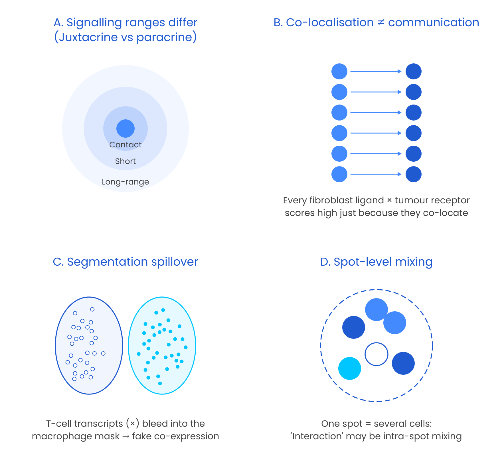
Figure 2: Four core difficulties in spatial CCC inference. (A) Signals act over very different ranges, from direct contact to long-range paracrine diffusion. (B) Co-located cell types appear to communicate even when they do not, because every ligand–receptor combination between them scores highly. (C) Imperfect segmentation assigns transcripts from one cell to its neighbour, producing artificial co-expression at boundaries. (D) Spot-based platforms average several cells into one measurement, blurring true interactions with within-spot mixing.

Explore with our experts

The early Era: Ligand–receptor scoring from dissociated cells

The first generation of CCC inference worked on dissociated single-cell RNA-seq and a simple premise: if one cell type expresses a ligand and another expresses its receptor, the two could be talking. Methods differed mainly in how they decided whether that co-expression was meaningful.

CellPhoneDB shuffles cell-type labels to build a permutation null and, importantly, insists that every subunit of a receptor complex is present. CellChat treats interaction probability as a mass-action process that also accounts for agonists and antagonists. NicheNet took a different and, in hindsight, prescient route: rather than scoring the pair, it asks which ligands best predict the target genes switched on in the receiver, using prior signalling and regulatory networks. As methods multiplied, LIANA+ benchmarked and unified them, and showed that the choice of method and database changes the answer more than most users would expect (Dimitrov et al., 2022).

This generation has reached impressive scale. The CellCommuNet atlas, for example, compiles communication networks from 376 scRNA-seq datasets covering 82 diseases and 35 tissues: about 4.3 million cells and 514,463 inferred networks (Ma et al., 2024). Yet its authors point out that spatial information is missing, that cell-type misannotation produces incorrect networks, and that external signals are overlooked.

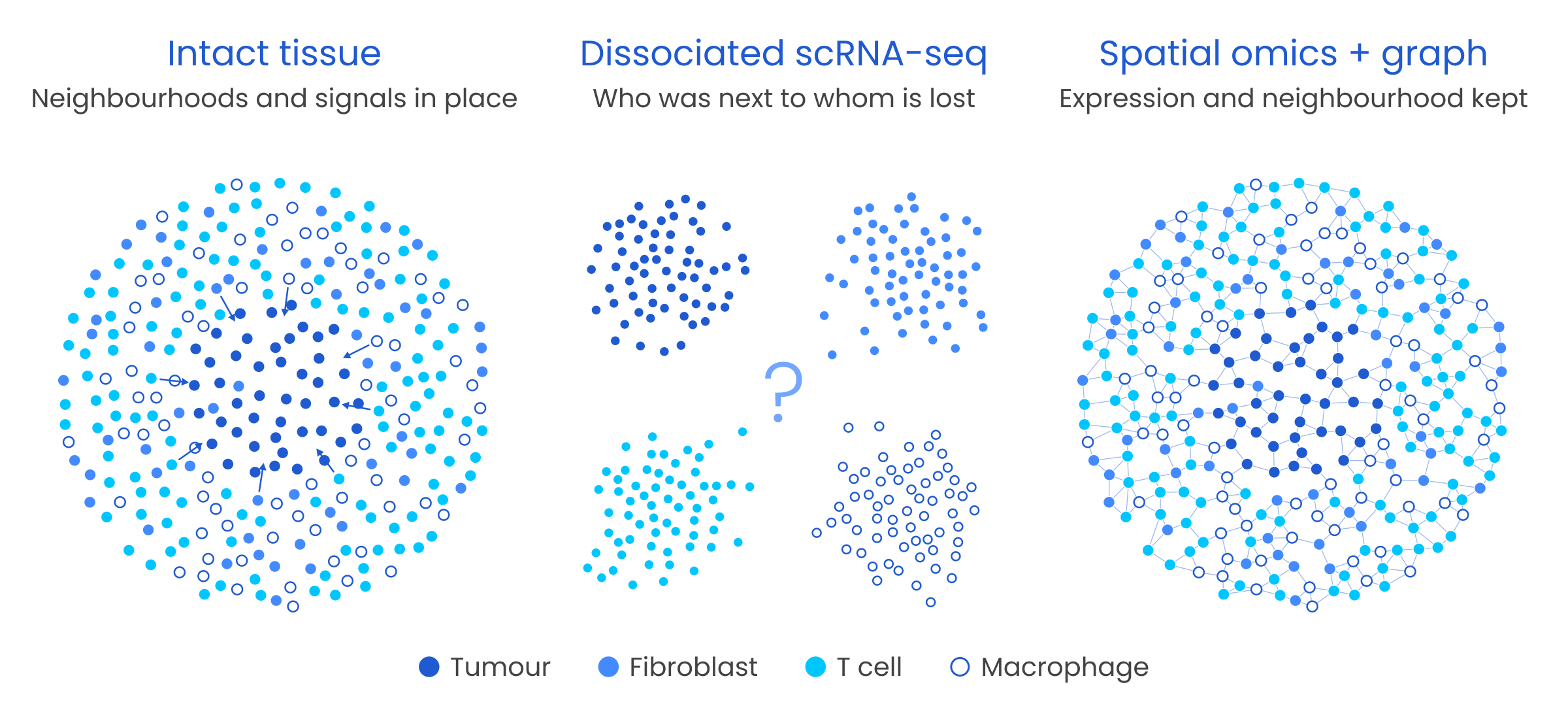
Figure 3: What dissociation loses. In intact tissue (left), tumour cells, fibroblasts, T cells and macrophages occupy structured neighbourhoods with directional signals. Dissociated scRNA-seq (middle) keeps each cell’s transcriptome but collapses the tissue into cell-type clusters, so who was next to whom is lost. Spatial omics (right) keeps expression and neighbourhood, which can be encoded as a cell graph for downstream modelling.

The ceiling of this era is structural, not methodological. Dissociation erases proximity, so no amount of clever scoring can separate cell types that merely coexist in a sample from cell types that actually touch. Results lean heavily on annotation quality, and nothing in the output shows that a receiver responded. These methods could list who might talk, but not who did.

Adding space: Spatial statistics and optimal transport

Spatial omics restored location, and the question became whether communication signals are structured in space.

The most direct answer is statistical. Bivariate spatial autocorrelation, as implemented in SpatialDM, tests whether ligand expression in one place tracks receptor expression in its surroundings, while neighbourhood enrichment in toolkits such as Squidpy tests whether cell types sit together more often than chance. Restricting scores to a biologically plausible distance adds a crude but useful notion of range.

Optimal transport reframes the problem physically. Signalling becomes the movement of “ligand mass” from senders to receivers, at a cost that grows with distance. COMMOT extends this to many ligands and receptors competing for one another and outputs directional signalling flows, so one can ask not only whether a pathway is active but which way it points.

These methods added physical range and direction. But a spatial pattern is still a pattern, and as Section 1 showed, tissue architecture alone can produce one. Nothing yet tests whether the receiver did anything.

From correlation to response: Receiver-centric models

The most important conceptual shift in the field is moving from

“Are the ligand and receptor near each other?” to “Does this signal explain what the receiving cell is doing?”

Receiver-centric models flip the direction of inference. Instead of scoring ligands, they model the receiver’s state and ask how much of it the surroundings explain. MISTy makes this explicit by splitting each gene’s variability into intracellular, juxtacrine and paracrine “views”: if the paracrine view adds nothing, there is little reason to claim paracrine signalling. NCEM predicts a cell’s expression from its neighbours on a spatial graph and reads sender → receiver effects off the fitted model, a short conceptual step from the GNNs in the next section. The same logic scales to cohorts: MultiNicheNet carries NicheNet’s ligand-to-target reasoning into multi-sample, multi-condition designs, and Tensor-cell2cell decomposes communication across samples into programmes that track disease state or outcome.

The common thread is that these models can be wrong in a measurable way. A claim that a signal explains a response can be checked on held-out cells and held-out sections, which is exactly what a co-expression score cannot offer.

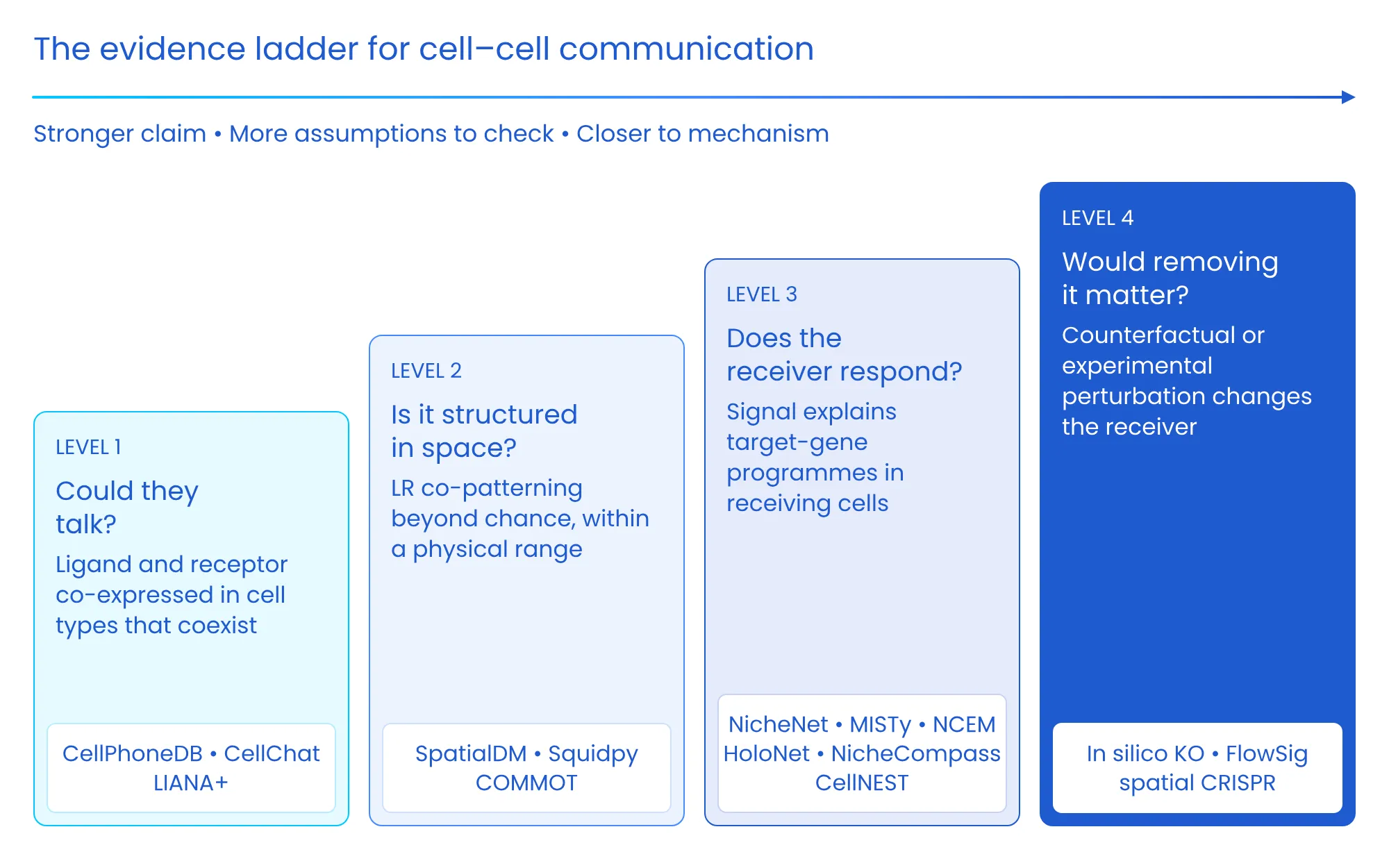
Figure 4: The evidence ladder for cell–cell communication. Each level supports a stronger biological claim but requires more assumptions to be checked. Level 1 asks whether cells could talk, based on ligand–receptor co-expression. Level 2 asks whether that co-expression is structured in space within a plausible signalling range. Level 3 asks whether the signal explains a response in receiving cells, which is where receiver-centric models and GNNs operate. Level 4 asks whether removing the signal would change the receiver, through counterfactual modelling or experimental perturbation.

The graph learning revolution

Graph Neural Networks (GNNs) brought a decisive change: instead of scoring pairs one at a time, they learn how a cell’s neighbourhood shapes its state, directly from the tissue graph. Tissue is a graph, and GNNs can learn context-dependent, non-linear and multi-hop effects that pairwise scores cannot capture, while still letting us build biological priors into the architecture.

Tissue as a graph

• Nodes: cells (or deconvolved spots)

• Node features: gene expression, cell type, morphology, protein

• Edges: cells that could interact, defined by k-nearest neighbours, a radius (~30–50 µm for contact, ~100–250 µm for paracrine) or pruned Delaunay triangulation

• Edge features: distance, shared membrane length, ligand–receptor-specific weights

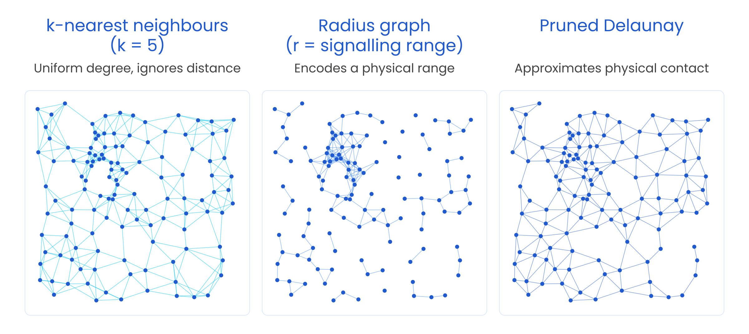
Figure 5: Three ways to turn a tissue section into a cell graph. k-nearest-neighbour graphs give every cell the same number of neighbours regardless of local density. Radius graphs encode an explicit physical signalling range. Pruned Delaunay triangulation approximates direct membrane contact and suits juxtacrine questions. The edge definition is itself a biological hypothesis and should be chosen deliberately and stress-tested.

Why message passing fits biology

A GNN layer updates each cell by aggregating “messages” from its neighbours:

$$h_i' = \phi\Big(h_i,\ \bigoplus_{j \in N(i)} \psi\big(h_i, h_j, e_{ij}\big)\Big)$$

• Message (ψ): the signal from sender j to receiver i, shaped by ligand, receptor and distance • Aggregation (⊕): the receiver integrates all incoming signals • Update (φ): the receiver changes state through target genes and pathways • Layers (L): the number of hops, which approximates signalling range (too many causes over-smoothing)

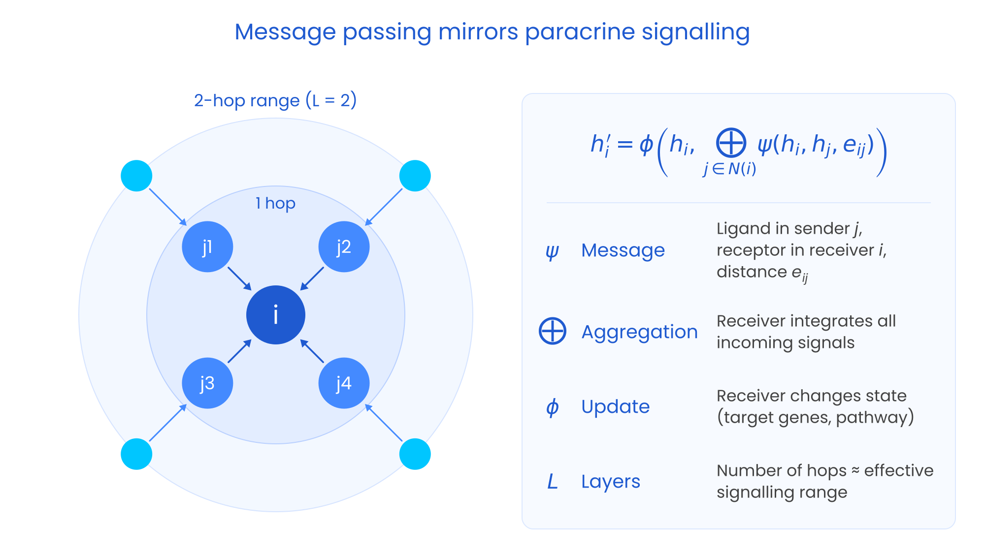
Figure 6: Message passing mirrors paracrine signalling. A receiver cell (i) collects messages from its direct neighbours (senders j₁–j₄). Each message can depend on ligand expression in the sender, receptor expression in the receiver and the distance between them. Second-hop cells (grey) influence the receiver indirectly through intermediate senders, so stacking L layers extends the effective signalling range to L hops.

The questions GNNs can answer

It is more useful to think about GNNs by the biological question they address than by architecture.

Which signals drive this response? Here the GNN is a receiver-response model. HoloNet builds one communication graph per ligand–receptor pair and uses attention to identify which pairs and which senders best explain a specific target gene in the receiver. This is the most direct route up the evidence ladder to Level 3.

What are the communication programmes of a niche? NicheCompass constrains its latent space so that each dimension corresponds to an interpretable communication programme. Niches can then be compared across samples and technologies, and the approach has been applied to an 8.4-million-cell mouse brain atlas.

Does signalling propagate beyond immediate neighbours? CellNEST uses graph attention to detect relay networks, chains in which a cell receives a signal and then sends a different one onward (ligand → receptor → ligand → receptor). DeepTalk pursues a similar single-cell-resolution goal with subgraph-based attention.

Which interactions are missing from our databases? Link-prediction models such as GCNG and DeepLinc propose new interacting gene pairs or cell interactions. Their output is a list of hypotheses, not evidence, and should enter the evidence ladder at Level 1.

Two supporting ingredients matter as much as the CCC model itself. Spatial-domain methods such as STAGATE, GraphST and BANKSY define where to test communication, so that comparisons are made within like-for-like tissue regions. And spatially aware foundation models such as Nicheformer, pretrained on more than 100 million cells, offer richer cell representations to use as node features.

Also read: The revolution in single-cell image analysis: From algorithms to agentic AI

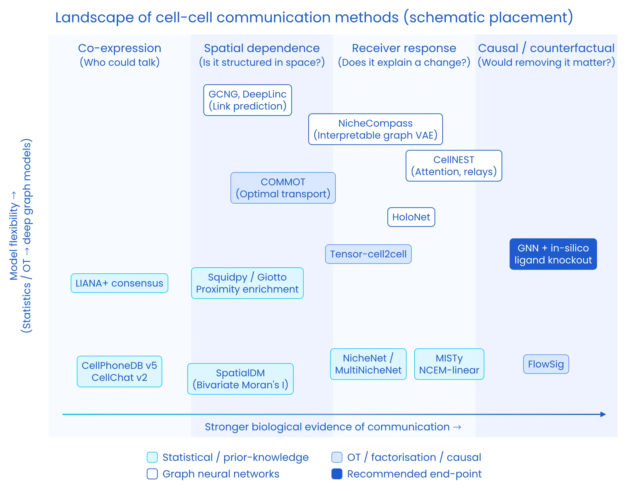
Figure 7: The landscape of cell–cell communication methods. The x-axis reflects the strength of biological evidence each approach provides, from co-expression to spatial dependence, receiver response and counterfactual testing. The y-axis reflects model flexibility, from statistical and optimal-transport methods to deep graph models. Statistical and prior-knowledge methods are shown in amber, optimal-transport, factorisation and causal methods in purple, and graph neural networks in teal. The recommended end-point, GNNs interrogated with in silico ligand knockouts, is shown in red. Placement is schematic.

Interrogate, Don’t Just Predict

A GNN that predicts expression accurately is not automatically telling us anything about communication. Its value comes from interrogating it:

• In silico ligand knockout: remove a ligand from senders and measure the predicted change in receivers

• Edge ablation: remove edges by distance or cell-type pair and observe the drop in performance

• Attribution: use GNNExplainer and integrated gradients to find the subgraph driving a prediction

• Stability checks: repeat across random seeds, graph constructions and held-out sections

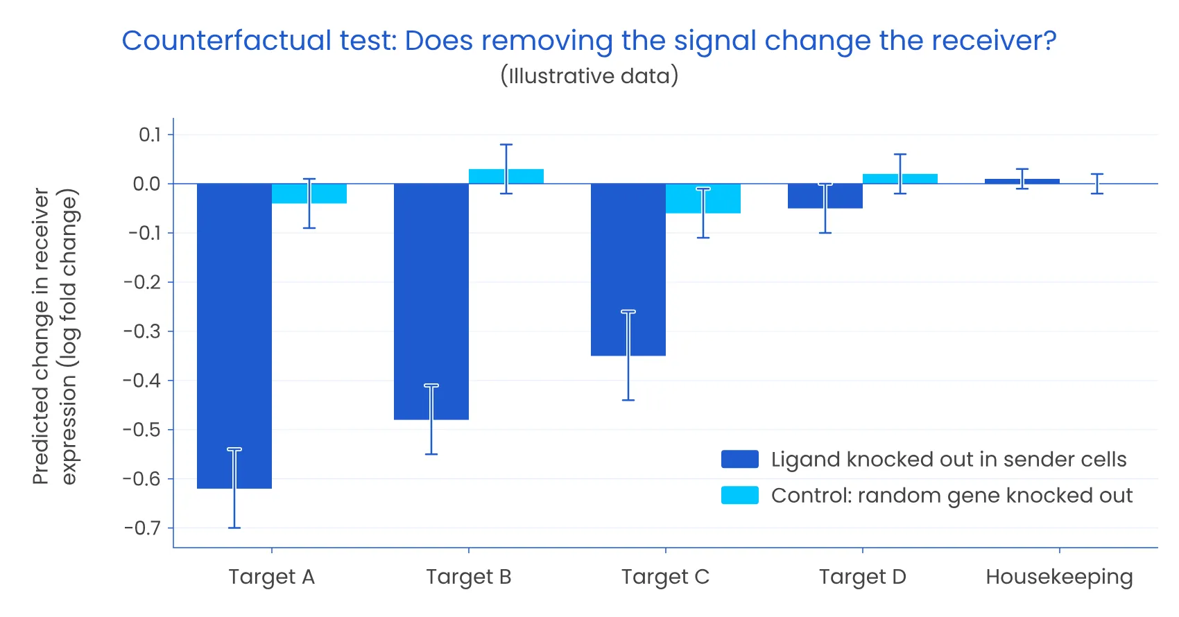
Figure 8: A counterfactual test for communication (illustrative data). When a ligand is knocked out in sender cells within a trained model, predicted expression of its downstream targets falls in receiving cells. A control knockout of a random gene and an unrelated housekeeping gene stay flat. A genuine interaction should pass this test; a co-location artefact usually will not.

Interrogated this way, GNNs move the field from co-expression to explained receiver response, capture multi-hop and relay signalling, combine biological priors with learned patterns, and scale to atlases of millions of cells.

But GNNs still lack judgement. Attention weights are not explanations, edge choices are hypotheses, and confounders do not disappear on their own.

Guarding against false discoveries

Whatever the model, the same safeguards apply:

• Condition on cell-type composition: does the ligand–receptor pair explain anything beyond co-location?

• Use spatially aware null models: permute within cell types or spatial domains, not globally

• Stress-test segmentation: compare against nucleus-only counts or an alternative segmenter such as Baysor

• Check panel coverage: confirm the ligand, all receptor subunits and key targets are measured

• Deconvolve spot data first: with Cell2location, RCTD or Tangram

• Verify cell annotation: misannotated cell types generate incorrect communication networks

• Validate orthogonally: with spatial proteomics, phospho-signalling or spatial CRISPR screens

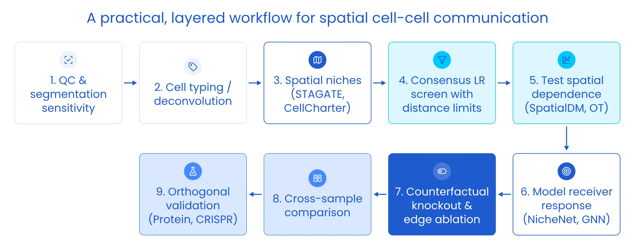
Figure 9: A practical, layered workflow for spatial cell–cell communication. Analysis begins with quality control and segmentation sensitivity, then cell typing or deconvolution and spatial niche definition. A consensus ligand–receptor screen with distance limits generates candidates, which are filtered by tests of spatial dependence and then explained with receiver-response models such as NicheNet or GNNs. Counterfactual knockouts and edge ablation test robustness, cross-sample comparison links communication to condition, and orthogonal validation confirms the strongest findings.

The next frontier: Agentic AI for cell–cell communication

Why CCC is an agent-shaped problem

Figure 9 looks linear on paper. In practice it is not. The right next step almost always depends on what the previous step found:

• If a juxtacrine hit disappears when you recount with nucleus-only transcripts, you do not escalate it to a GNN. You drop it, or you go back and re-segment.

• If the panel is missing a receptor subunit, the question changes: that pathway can never rise above Level 1 in this dataset, however good the model.

• If an effect appears in four of twelve samples, the interesting question is no longer “is there an effect?” but “what do those four have in common?”

Workflow managers such as Snakemake and Nextflow are excellent at executing a plan that has already been decided. The hard part of CCC analysis is deciding, dozens of times, with each decision conditional on intermediate results. Today that judgement lives in an expert’s head. It is slow, it varies between analysts, and it is rarely written down, which is why two groups can analyse the same dataset and report different networks.

That is the gap agentic AI can fill: not writing analysis code faster, but making conditional decisions across a long chain of steps, and recording why each one was made.

Anatomy of a CCC agent

An agent is not a chatbot that writes Scanpy code. It is a system that holds a goal, plans, calls tools, observes the results and changes course. For CCC, four roles are useful:

• Planner: turns a biological question into a written analysis plan, including which pathways to test, the signalling range assumed for each, and the graph construction that follows from that range

• Tool agents: wrap well-tested methods (consensus ligand–receptor screens, spatial statistics, optimal transport, GNN response models) behind typed interfaces with explicit inputs and outputs

• Critic: applies the safeguards from Section 6 to every candidate before it can be reported, and sends work back to the planner when a check fails

• Evidence ledger: a structured record of every claim, the evidence level it reached on the ladder in Figure 4, the checks it passed or failed, and every analysis branch that was tried

Explore our AI solutions

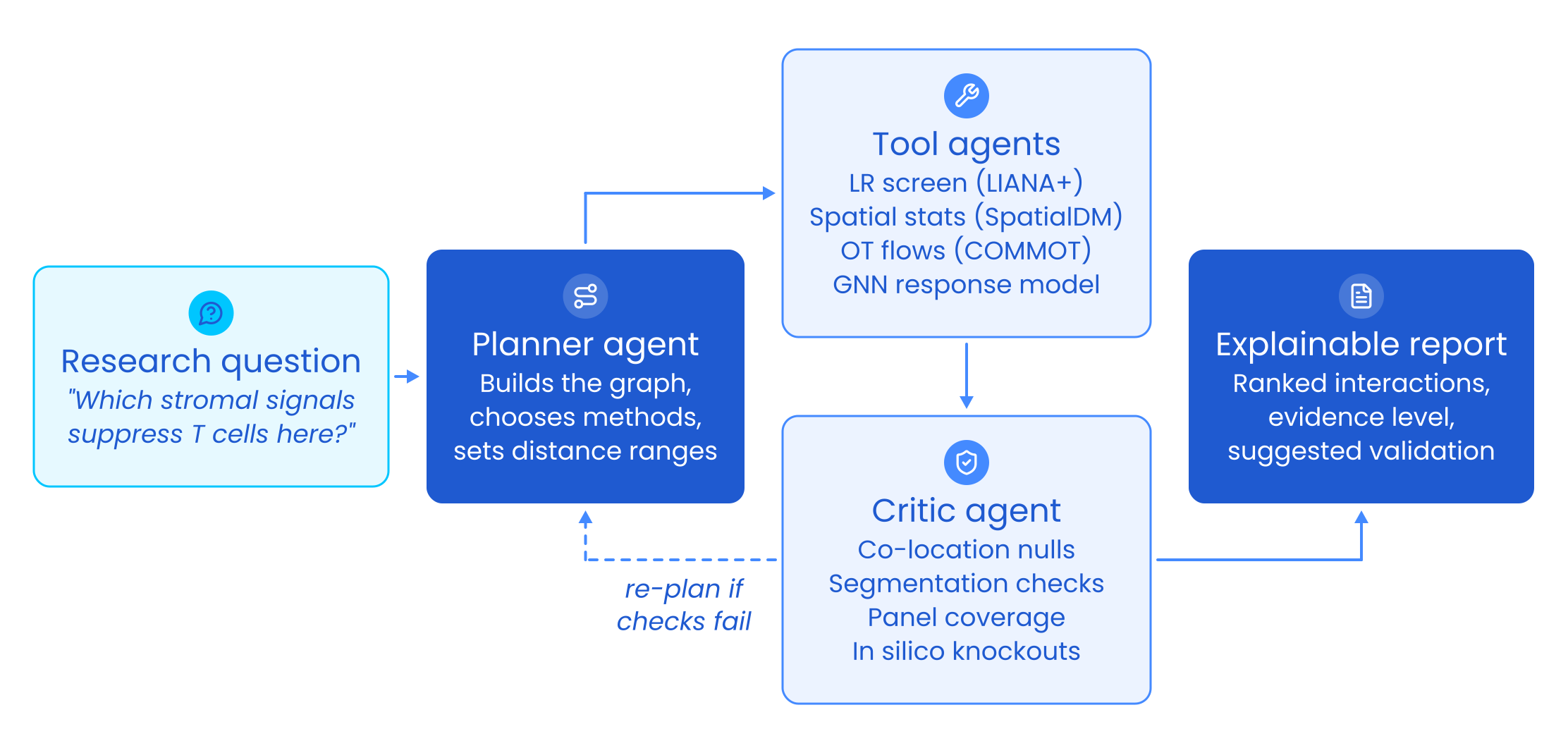
Figure 10: An example of an agentic reasoning framework for cell–cell communication. A research question is translated by a planner agent into an analysis plan: graph construction, method selection and distance ranges. Tool agents run consensus ligand–receptor screening, spatial statistics, optimal-transport flows and GNN response models. A critic agent tests every candidate against co-location nulls, segmentation sensitivity, panel coverage and in silico knockouts, and sends the plan back for revision if checks fail. The output is an explainable report ranking interactions by evidence level and suggesting validation experiments.

A worked example: One question, end to end

To make this concrete, consider a hypothetical study: twelve imaging-based spatial transcriptomics sections from colorectal tumours, and the question “Do cancer-associated fibroblasts (CAFs) keep CD8 T cells out of tumour nests, and if so, through which signals?” The trace below is illustrative, not a real result, but each step reflects a decision an analyst would otherwise make by hand.

Step	Role	What happens	Outcome
1	Planner	Defines CAF and CD8 T-cell populations and a response variable (T-cell distance into tumour nests). Lists candidate pathways and assigns each a range: chemokines and TGF-β as paracrine (~150 µm radius graph), checkpoint ligands as contact (pruned Delaunay). Writes the plan to the ledger before any results are seen.	Pre-registered plan
2	Tool + Critic	Audits panel coverage for every ligand, receptor subunit and key target gene.	One TGF-β receptor subunit is missing, so that pathway is capped at Level 1 and flagged
3	Tool	Runs a consensus ligand–receptor screen with the pathway-specific distance limits.	40 candidate CAF → T-cell interactions
4	Critic	Tests each candidate against a co-location null conditioned on cell-type composition, then repeats contact candidates with nucleus-only counts.	31 explained by CAFs simply surrounding tumour nests; 2 contact hits vanish without cytoplasmic transcripts. 9 survive
5	Tool	Fits a GNN receiver-response model for the T-cell state and runs in silico knockouts of each surviving ligand, with random-gene controls.	3 ligands produce knockout effects clearly above control
6	Critic → Planner	Notices the strongest effect appears in only 4 of 12 sections. Rather than report a pooled effect, the planner adds a stratified analysis by available clinical covariates.	Effect tracks one tumour subtype; a human reviewer is asked to confirm the stratification is biologically sensible
7	Reporter	Generates the report from the ledger, not from free text.	3 interactions at Level 3, each with its checks, the branches tried, and a suggested validation (protein staining for the ligand, receptor blockade in a co-culture model)

Two things stand out. First, most of the agent’s value comes from eliminating candidates, not finding them: 37 of 40 were removed for documented reasons. Second, every elimination is auditable, so a biologist who disagrees with a decision can see exactly where to push back.

Design principles for a trustworthy agent

The language model decides; code computes. Statistics, nulls and knockouts run in deterministic, versioned tools. The model chooses which tool to call and interprets the result, but never estimates a p-value or an effect size itself.

Hard checks cannot be argued away. The critic should be mostly not a language model. Co-location nulls, segmentation sensitivity, panel coverage and knockout-versus-control comparisons are coded checks with explicit thresholds. A language-model critic can add a layer of biological plausibility review on top, but it cannot overturn a failed hard check.

Language is capped by evidence. Because the report is generated from the ledger, the wording is tied to the evidence level. A Level 2 interaction can be described as “spatially co-expressed within signalling range”; it cannot be described as “CAFs signal to T cells”. This single rule removes much of the over-claiming that creeps into CCC papers.

Guard against automated p-hacking. An agent that can try twenty graph constructions and five null models in an hour is a garden of forking paths running at machine speed (Gelman & Loken, 2014). Left unchecked, it will find something. The defences are the same as in good human science, applied rigorously: pre-register the plan, log every branch including the failed ones, correct for multiple testing across the agent’s whole search, and report findings that are robust across reasonable choices (a multiverse analysis; Steegen et al., 2016) rather than the single best-looking result.

Keep humans at the decisions that encode biology. Cell-type annotation, the choice of candidate pathways, stratification variables and any claim at Level 3 or above are natural checkpoints for expert review. Corrections made there should be stored and reused, so the agent improves with each project rather than repeating the same mistakes.

Ground knowledge in sources. Ligand–receptor pairs, complex compositions and typical signalling ranges should come from curated resources and the literature, retrieved and cited, not from the model’s memory. When the agent has to make an assumption that no resource supports, the ledger should say so.

How do we know it works?

Agents need benchmarks as much as models do, and CCC has a natural one: simulated tissues with planted ground truth. A simulator can place cells in realistic architectures, plant interactions with known senders, ranges and target-gene effects, and then add the traps from Section 1: co-located cell types that do not communicate, segmentation spillover at boundaries, and panels missing a receptor subunit.

An agent can then be scored on questions that matter in practice:

• Recall: does it recover the planted interactions?

• Trap avoidance: how many co-location and spillover artifacts does it report?

• Calibration: do its evidence levels match the truth?

• Escalation: does it ask a human at the right moments, and not at every step?

• Reproducibility: does the same question on the same data give the same conclusions twice?

Simulation is necessary but not sufficient. Real datasets with known biology, and especially spatial perturbation data such as Perturb-map spatial CRISPR screens (Dhainaut et al., 2022), provide a harder test: did the agent’s Level 3 claims hold up when the signal was actually removed?

Early general-purpose systems show the building blocks are within reach. Biomni demonstrates an agent chaining a broad set of biomedical tools and databases, and BioDiscoveryAgent shows an agent iteratively designing genetic perturbation experiments from previous results. CCC is an especially good target for a specialized agent because its failure modes are already well cataloged and can be written down as checks. The most exciting version closes the loop: the agent proposes the perturbation that would move a claim from Level 3 to Level 4, the experiment is run, and the result updates the model.

Where agents can still go wrong

Agents introduce failure modes of their own. Language models can confidently pair the wrong receptor with a ligand, or construct a fluent biological narrative around a weak result. They can over-trust a tool’s default parameters, or quietly drop a failing branch. Long runs are expensive and hard to debug. None of these is a reason to avoid agents, but each is a reason to insist on the principles above: deterministic tools, hard checks, evidence-capped language and a complete ledger. An agent that cannot show its working is no better than an unreviewed pipeline.

An Infocusp perspective: Build the test bench before the agent

At Infocusp we build AI systems that have to work outside a notebook, for life-science teams and for other domains where a wrong answer is expensive. Looking at spatial CCC through that engineering lens, our view is simple: the model is rarely the bottleneck; the decisions around it are.

Graph construction, segmentation, annotation and null models each move the answer more than swapping one GNN architecture for another. So if we were starting a CCC programme today, we would build in this order:

1. The test bench first. A tissue simulator with planted interactions and planted artifacts is the CCC equivalent of a unit-test suite. Without it, there is no way to tell whether a change to the pipeline, the model or the agent made things better or merely different.
2. Sensitivity analysis as infrastructure, not an afterthought. Re-running an analysis across segmentations, graph definitions and seeds should be one command. Once it is cheap, it stops being skipped.
3. The agent last, and auditable to a biologist. The deliverable is not a network diagram. It is an evidence ledger a wet-lab scientist can challenge, and a short list of interactions worth taking to the bench.

We would also change what success looks like. The number of interactions an analysis reports says little about its quality. A better measure is the validation hit rate: of the interactions sent for experimental follow-up, how many held up? An agent that reports five interactions, three of which validate, is worth far more than one that reports fifty.

Conclusion: From co-expression to causal understanding

The future of cell–cell communication analysis is not about scoring more ligand–receptor pairs. It is about asking better questions of tissue as a system.

We are moving toward:

• Physics-informed graph models that build production, diffusion and consumption into message functions, bridging statistical inference with physicochemical mechanism

• Causal models trained on spatial perturbation screens

• Multimodal graphs that integrate chromatin, protein, metabolites and histology

• Agentic systems that plan, test and explain analyses end to end, record every decision, and propose the experiments that would prove them wrong

This evolution mirrors the broader trajectory of AI in science:

From listing → to locating → to explaining → to reasoning

Graph neural networks, grounded in biology and interrogated counterfactually, are bridging the gap between spatial snapshots and mechanistic understanding. Agentic systems, held to the same evidence standards, can make that rigor routine rather than heroic. Together they let us ask not just “what are these cells?” but “who is influencing whom, and what would change if that conversation stopped?”

The conversation between cells is finally becoming legible, and the most exciting discoveries are yet to come.

Explore with our experts

---

All figures are schematic illustrations created for this article. Figure 8 uses illustrative, not experimental, data. The worked example in Section 7 is a hypothetical scenario, not a reported result.

Appendix: Method quick reference

Question you are asking	Highest evidence level	Example methods
Could these cell types talk?	Level 1	CellPhoneDB, CellChat, LIANA+
Is the signal structured in space, and in which direction?	Level 2	SpatialDM, Squidpy, Giotto, COMMOT, SpaOTsc
Does the signal explain the receiver’s state?	Level 3	NicheNet, MultiNicheNet, MISTy, NCEM, HoloNet
What are the communication programmes of a niche, across samples?	Level 3	NicheCompass, Tensor-cell2cell
Does signalling relay across chains of cells?	Level 3	CellNEST, DeepTalk
Which new interactions should we hypothesise?	Level 1 (hypotheses)	GCNG, DeepLinc
Where in the tissue should we compare?	Supporting	STAGATE, GraphST, CellCharter, BANKSY, Nicheformer
Would removing the signal change the receiver?	Level 4	In silico knockouts on a trained response model; spatial CRISPR screens such as Perturb-map

References

1. Su J, Song Y, Zhu Z, et al. Cell–cell communication: new insights and clinical implications. Signal Transduct Target Ther. 2024;9:196. https://doi.org/10.1038/s41392-024-01888-z?utm_source=Infocusp_Innovations&utm_medium=Blog
2. Luthria G, Lauffenburger D, Miller MA. Cell–cell communication networks in tissue: toward quantitatively linking structure with function. Curr Opin Syst Biol. 2021;27:100341. https://doi.org/10.1016/j.coisb.2021.05.002?utm_source=Infocusp_Innovations&utm_medium=Blog
3. Ma Q, Li Q, Zheng X, Pan J. CellCommuNet: an atlas of cell–cell communication networks from single-cell RNA sequencing of human and mouse tissues in normal and disease states. Nucleic Acids Res. 2024;52(D1):D597–D606. https://doi.org/10.1093/nar/gkad906?utm_source=Infocusp_Innovations&utm_medium=Blog
4. Armingol E, Officer A, Harismendy O, Lewis NE. Deciphering cell–cell interactions and communication from gene expression. Nat Rev Genet. 2021;22:71–88.
5. Efremova M, Vento-Tormo M, Teichmann SA, Vento-Tormo R. CellPhoneDB: inferring cell–cell communication from combined expression of multi-subunit ligand–receptor complexes. Nat Protoc. 2020;15:1484–1506.
6. Jin S, Guerrero-Juarez CF, Zhang L, et al. Inference and analysis of cell-cell communication using CellChat. Nat Commun. 2021;12:1088.
7. Browaeys R, Saelens W, Saeys Y. NicheNet: modeling intercellular communication by linking ligands to target genes. Nat Methods. 2020;17:159–162.
8. Dimitrov D, Türei D, Garrido-Rodriguez M, et al. Comparison of methods and resources for cell-cell communication inference from single-cell RNA-Seq data. Nat Commun. 2022;13:3224.
9. Dimitrov D, Schäfer PSL, Farr E, et al. LIANA+ provides an all-in-one framework for cell–cell communication inference. Nat Cell Biol. 2024;26:1613–1622.
10. Li Z, Wang T, Liu P, Huang Y. SpatialDM for rapid identification of spatially co-expressed ligand–receptor and revealing cell–cell communication patterns. Nat Commun. 2023;14:3995.
11. Cang Z, Zhao Y, Almet AA, et al. Screening cell–cell communication in spatial transcriptomics via collective optimal transport. Nat Methods. 2023;20:218–228.
12. Tanevski J, Ramirez Flores RO, Gabor A, Schapiro D, Saez-Rodriguez J. Explainable multiview framework for dissecting spatial relationships from highly multiplexed data. Genome Biol. 2022;23:97.
13. Fischer DS, Schaar AC, Theis FJ. Modeling intercellular communication in tissues using spatial graphs of cells. Nat Biotechnol. 2023;41:332–336.
14. Armingol E, Baghdassarian HM, Martino C, et al. Context-aware deconvolution of cell–cell communication with Tensor-cell2cell. Nat Commun. 2022;13:3665.
15. Li H, Ma T, Hao M, Wei L, Zhang X. Decoding functional cell–cell communication events by multi-view graph learning on spatial transcriptomics (HoloNet). bioRxiv. 2022. https://doi.org/10.1101/2022.06.22.496105?utm_source=Infocusp_Innovations&utm_medium=Blog
16. Birk S, Bonafonte-Pardàs I, Feriz AM, et al. Quantitative characterization of cell niches in spatially resolved omics data (NicheCompass). Nat Genet. 2025;57:897–909.
17. Zohora FT, Paliwal D, Flores-Figueroa E, et al. CellNEST reveals cell–cell relay networks using attention mechanisms on spatial transcriptomics. Nat Methods. 2025;22:1505–1519. https://doi.org/10.1038/s41592-025-02721-3?utm_source=Infocusp_Innovations&utm_medium=Blog
18. Yang W, Wang P, Xu S, et al. Deciphering cell–cell communication at single-cell resolution for spatial transcriptomics with subgraph-based graph attention network (DeepTalk). Nat Commun. 2024;15. https://doi.org/10.1038/s41467-024-51329-2?utm_source=Infocusp_Innovations&utm_medium=Blog
19. Yuan Y, Bar-Joseph Z. GCNG: graph convolutional networks for inferring gene interaction from spatial transcriptomics data. Genome Biol. 2020;21:300.
20. Li R, Yang X. De novo reconstruction of cell interaction landscapes from single-cell spatial transcriptome data with DeepLinc. Genome Biol. 2022;23:124.
21. Tejada-Lapuerta A, Schaar AC, et al. Nicheformer: a foundation model for single-cell and spatial omics. Nat Methods. 2025. https://doi.org/10.1038/s41592-025-02814-z?utm_source=Infocusp_Innovations&utm_medium=Blog
22. Dong K, Zhang S. Deciphering spatial domains from spatially resolved transcriptomics with an adaptive graph attention auto-encoder. Nat Commun. 2022;13:1739.
23. Gilmer J, Schoenholz SS, Riley PF, Vinyals O, Dahl GE. Neural message passing for quantum chemistry. Proc ICML. 2017.
24. Ying R, Bourgeois D, You J, Zitnik M, Leskovec J. GNNExplainer: generating explanations for graph neural networks. Proc NeurIPS. 2019.
25. Jain S, Wallace BC. Attention is not explanation. Proc NAACL. 2019.
26. Almet AA, Tsai YC, Watanabe M, Nie Q. Inferring pattern-driving intercellular flows from single-cell and spatial transcriptomics (FlowSig). Nat Methods. 2024;21:1806–1817.
27. Dhainaut M, Rose SA, Akturk G, et al. Spatial CRISPR genomics identifies regulators of the tumor microenvironment (Perturb-map). Cell. 2022;185:1223–1239.
28. Oyler-Yaniv A, Oyler-Yaniv J, Whitlock BM, et al. A tunable diffusion-consumption mechanism of cytokine propagation enables plasticity in cell-to-cell communication in the immune system. Immunity. 2017;46:609–620.
29. Gelman A, Loken E. The statistical crisis in science. Am Sci. 2014;102(6):460–465. https://doi.org/10.1511/2014.111.460?utm_source=Infocusp_Innovations&utm_medium=Blog
30. Steegen S, Tuerlinckx F, Gelman A, Vanpaemel W. Increasing transparency through a multiverse analysis. Perspect Psychol Sci. 2016;11(5):702–712. https://doi.org/10.1177/1745691616658637?utm_source=Infocusp_Innovations&utm_medium=Blog
31. Huang K, Zhang S, Wang H, et al. Biomni: a general-purpose biomedical AI agent. bioRxiv. 2025. https://doi.org/10.1101/2025.05.30.656746?utm_source=Infocusp_Innovations&utm_medium=Blog
32. Roohani Y, Lee A, Huang Q, et al. BioDiscoveryAgent: an AI agent for designing genetic perturbation experiments. Proc ICLR. 2025. https://arxiv.org/abs/2405.17631?utm_source=Infocusp_Innovations&utm_medium=Blog