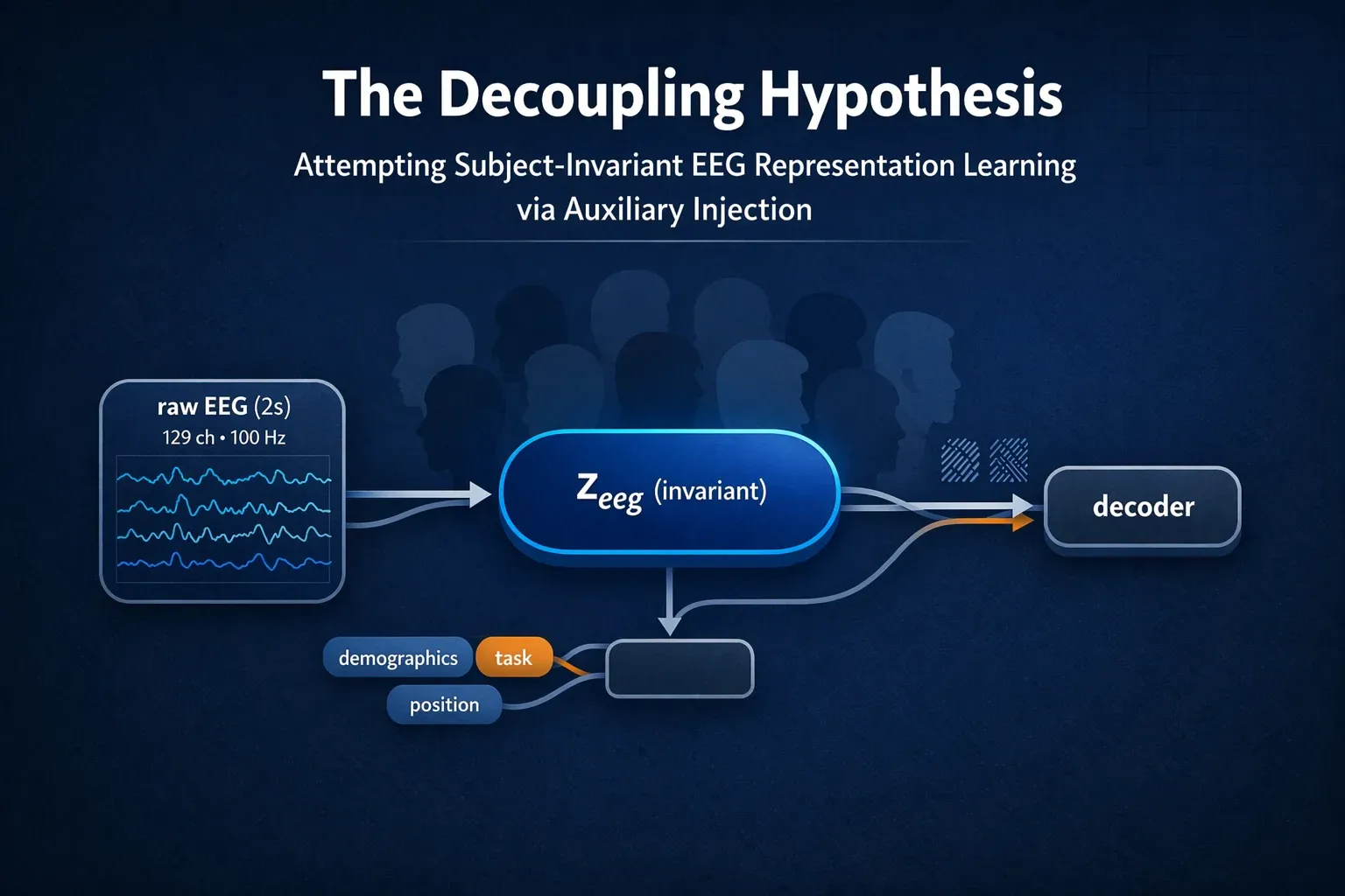
The Decoupling Hypothesis: Attempting Subject-Invariant EEG Representation Learning via Auxiliary Injection

Overview

Decoding the human brain is difficult; decoding it from short, noisy snippets of electrical activity is even harder.

We participated in the NeurIPS 2025 EEG Foundation Challenge, where the goal was to predict behavioral metrics (reaction time) and clinical diagnostics (psychopathology factors) from only 2-second windows of raw EEG.

Our team reached:

• Rank 54 in Challenge 1 (Reaction Time Prediction)
• Rank 16 in Challenge 2 (Psychopathology Prediction)

The core research problem we tackled was subject invariance. EEG models can overfit to subject-specific artifacts (for example skull thickness, hair density, and age-related signal differences) rather than learning neural dynamics that generalize across participants.

A 2-second window at 100 Hz has only 200 samples. This is enough to capture faster oscillations (such as alpha and beta), but it limits robust modeling of slower dynamics tied to fatigue, engagement drift, or long-range task progression.

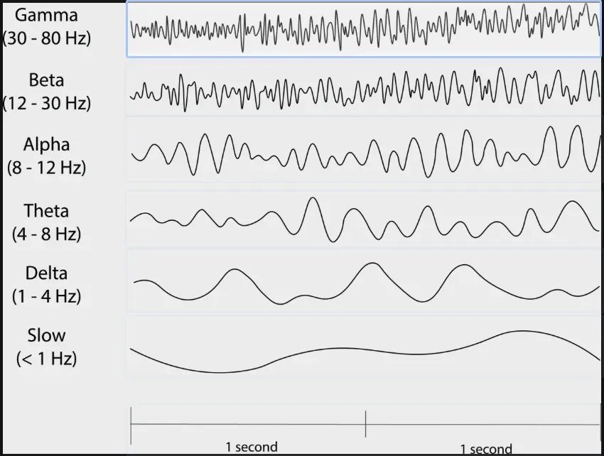Figure 1. Visualization of common brainwave frequency bands.

Our central idea was straightforward:

• Let the encoder see only the raw 2-second EEG segment.
• Give the decoder additional nuisance/context variables (demographics, task identity, sequence position).
• Force the encoder to prioritize invariant neural content while the decoder handles context-heavy reconstruction details.

In short, we tried to approximate long-range context modeling without using expensive RNN/Transformer sequence models.

---

The HBN Dataset and Challenge Setup

The competition used the Healthy Brain Network (HBN) EEG dataset with recordings from over 3,000 participants across six tasks.

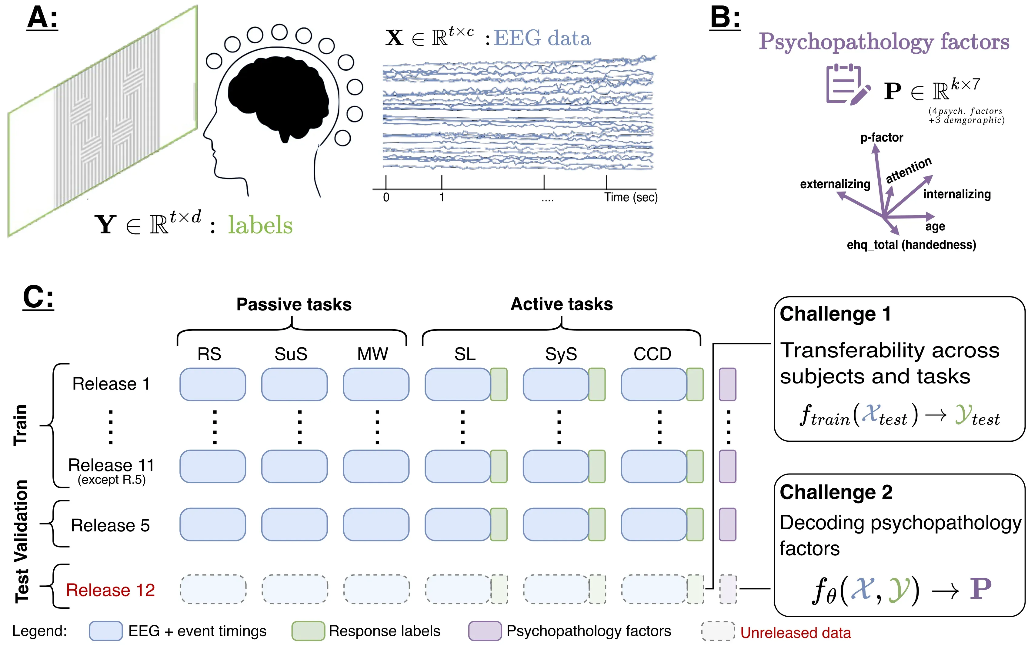Figure 2. HBN-EEG dataset overview and train/validation/test split.

Task groups

1. Passive tasks (sensory processing):
   • Resting State (RS)
   • Surround Suppression (SuS)
   • Movie Watching (MW)
2. Active tasks (cognitive load + response):
   • Contrast Change Detection (CCD)
   • Sequence Learning (SL)
   • Symbol Search (SyS)

Prediction targets

• Reaction time
• Four psychopathology factors

Input constraints

• Window length: 2 seconds
• Sampling rate: 100 Hz
• Channels: 129 (128 EEG + 1 reference)
• No preprocessing allowed (artifact filtering, denoising, normalization had to be learned by the model)

This yields a key question:

Can we learn subject-invariant and task-robust EEG embeddings from only 2 seconds of raw signal?

---

Related SSL Landscape and Our Positioning

Recent EEG self-supervised learning usually falls into several families:

• Masked reconstruction (MAE-style masking and reconstruction)
• Contrastive learning (SimCLR/CPC-style objectives with EEG-specific augmentations)
• Bootstrap/teacher-student methods (BYOL/VICReg-style objectives without explicit negatives)
• Prototype or clustering-based SSL
• Foundation-model approaches that combine multiple SSL objectives

Our method was not a pure SSL foundation model. It was a practical competition-time architecture designed around a decoupling hypothesis: inject nuisance/context only where needed for reconstruction, and pressure the main latent to become more invariant.

---

Core Methodology

1) Encoder input preparation

Given raw EEG tensor:

X ∈ R^(B x 129 x 200)

we split channels into 128 signal channels and 1 reference channel, broadcast the reference channel across 128 channels, and stack to obtain:

X' ∈ R^(B x 128 x 200 x 2)

2) Multi-scale temporal feature extraction

We used parallel convolutions with kernel sizes [1, 15, 45] to cover immediate, medium-scale, and slower temporal patterns:

H_0 = Concat(H_{k=1}, H_{k=15}, H_{k=45})

3) Dual dilated branches with orthogonality pressure

Two additional convolution branches with dilation schedules (1, 2, 4, 16) were used to capture diverse temporal dependencies.

We encouraged feature diversity with:

L_ortho = || H1^T · H2 ||_F^2

where flattened branch features are compared via Frobenius norm.

Figure 3. Proposed architecture with auxiliary injection into the decoder pathway. Architecture diagram designed using claude sonnet 4.6

4) Auxiliary injection for disentanglement

Auxiliary features included:

• Demographics (age, sex, handedness)
• Coarse task identity
• Sequence-position features (linear, exponential, sinusoidal variants)

A small MLP encoded this to a 32D vector:

z_aux = f_θ( [d_demo, p_pos, t_task] )

Main path:

z_eeg = E(x_raw)

Reconstruction path:

x_hat = D( Concat(z_eeg, z_aux) )

Key training asymmetry:

• Dropout applied to z_eeg
• No dropout applied to z_aux

This was intended to make the decoder rely on auxiliary context for easy, static reconstruction cues, while forcing the encoder to preserve more invariant neural information.

5) Spatial scaling using electrode geometry

Let D_norm,c be normalized electrode distance from a center. We scaled channel latents by inverse distance:

Z'_c = Z_c · 1 / (D_norm,c + ε)

This acted as a soft spatial reweighting mechanism before downstream dense blocks.

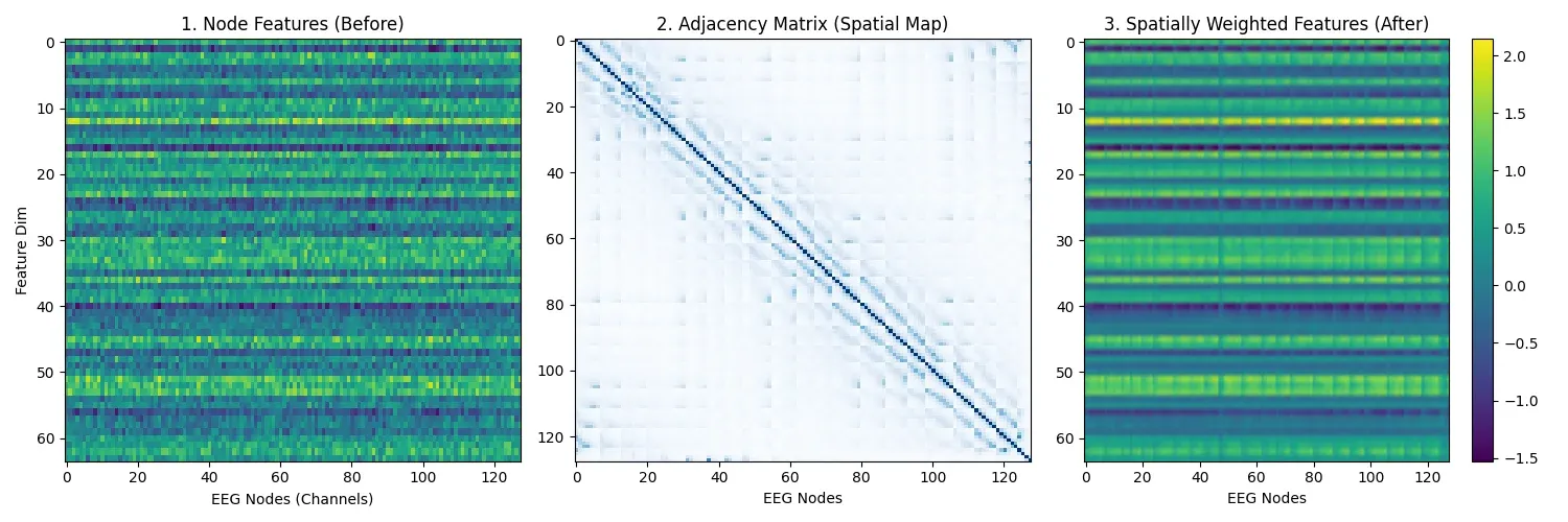Figure 4. Before/after visualization of spatial reweighting effects.

6) Multi-task pseudo-label supervision

To regularize representation quality, we added task-specific auxiliary heads using known metadata-derived pseudo-labels.

Examples:

• Contrast Change: side/contrast correctness/reaction-time related labels
• Sequence Learning: correctness counts, target counts, phase labels
• Resting State: eyes-open vs eyes-closed segments
• Movie task: movie segment identifiers

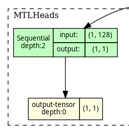Figure 5. Task-specific prediction head used for pseudo-label supervision.

---

Objective Function

Total training loss:

L_total = λ_recon · L_recon
   + λ_scl   · L_scl
   + λ_mtl   · L_mtl
   + λ_ortho · L_ortho

with weights:

• λ_recon = 1.0
• λ_mtl = 1.0
• λ_scl = 0.001
• λ_ortho = 0.1

Loss terms:

• Reconstruction loss (MSE)
• Supervised contrastive loss
• Multi-task pseudo-label loss (masked mixture of BCE/MSE/Cross-Entropy)
• Orthogonality regularization

---

Results and Retrospective

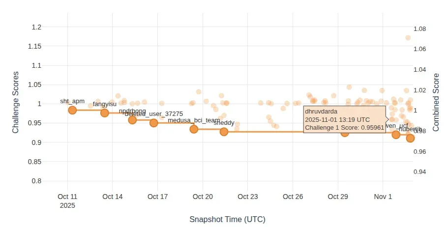Figure 6. Challenge 1 ranking snapshot around our submission.

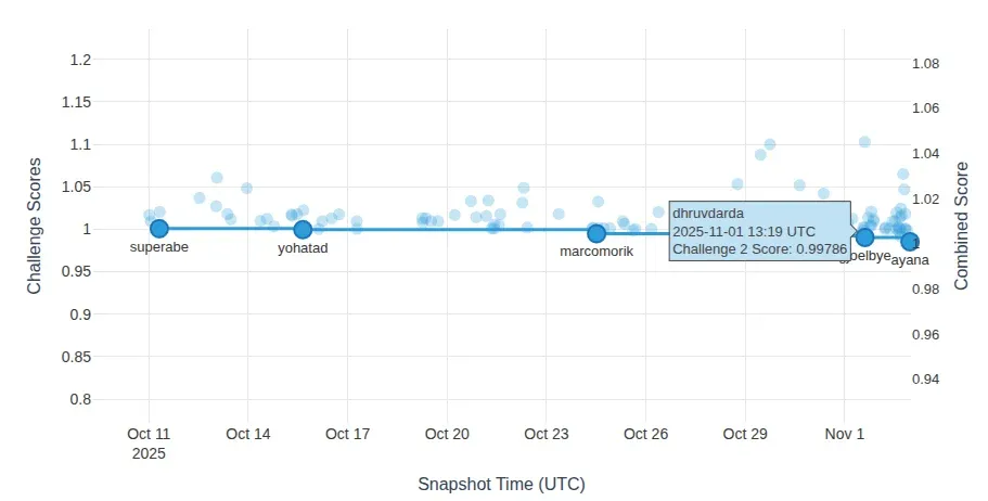Figure 7. Challenge 2 ranking snapshot around our submission.

Metric	Our Score	Top Score	Rank
Challenge 1 (Reaction Time)	0.95961	0.88668	54
Challenge 2 (Psychopathology)	0.99786	0.97843	16

What did not work as intended

1. Manual positional features were too simplistic. Real cognitive drift and fatigue are non-linear and state-dependent, so handcrafted ramps/decays were often mismatched to actual dynamics.

2. Demographic disentanglement was harder than expected. Demographic effects influence more than amplitude; they alter spectrum and coupling structure. Simple decoder-side concatenation was not expressive enough to fully isolate these effects.

3. Orthogonality was likely too strict. EEG features are naturally correlated. Strong decorrelation pressure can suppress useful redundancy.

---

What We Would Try Next

1. Evaluate the same ideas on full held-out test labels to confirm robustness claims.
2. Replace handcrafted position signals with learnable time embeddings.
3. Replace heuristic spatial scaling with graph-based modeling (for example GAT over electrode topology).
4. Explore stronger disentanglement objectives (adversarial nuisance removal, conditional priors, or factorized latents).

---

References

• Aristimunha et al. (2025). EEG Foundation Challenge: From Cross-Task to Cross-Subject EEG Decoding. arXiv:2506.19141. https://arxiv.org/abs/2506.19141
• Alexander et al. (2017). An open resource for transdiagnostic research in pediatric mental health and learning disorders. Scientific Data.
• Khosla et al. (2020). Supervised Contrastive Learning. NeurIPS.
• Weng (2023). Self-supervised Learning for Electroencephalogram: A Systematic Survey. ACM Computing Surveys.
• Ding and Wu (2023). Self-Supervised Learning for Biomedical Signal Processing. Biomedical Signal Processing and Control.
• He et al. (2022). Masked Autoencoders Are Scalable Vision Learners. CVPR.
• Chen et al. (2020). A Simple Framework for Contrastive Learning of Visual Representations. ICML.
• van den Oord et al. (2018). Representation Learning with Contrastive Predictive Coding. arXiv:1807.03748.
• Eldele et al. (2021). Temporal Contrastive Self-Supervised Learning for Time Series. AAAI.
• Banville et al. (2021). Self-supervised Representation Learning from EEG Signals. Journal of Neural Engineering.
• Grill et al. (2020). Bootstrap Your Own Latent. NeurIPS.
• Bardes et al. (2022). VICReg. ICLR.
• Yang et al. (2021). Prototype-Based Contrastive Learning for Time Series. arXiv:2105.08170.
• Zhang et al. (2024). EEGPT: Pretrained Transformer for EEG. arXiv:2406.07496.
• Li et al. (2023). BC-SSL: A Broad-Context Self-Supervised Learning Framework for EEG. arXiv:2310.06790.

I have also used LLMs for restructuring, and rephrasing, but the core ideas, technical direction, and learning are my own. The mathematical equations explaining loss functions are also generated using LLMs.