The Unpredictable Mind of an LLM — and How to Tame It

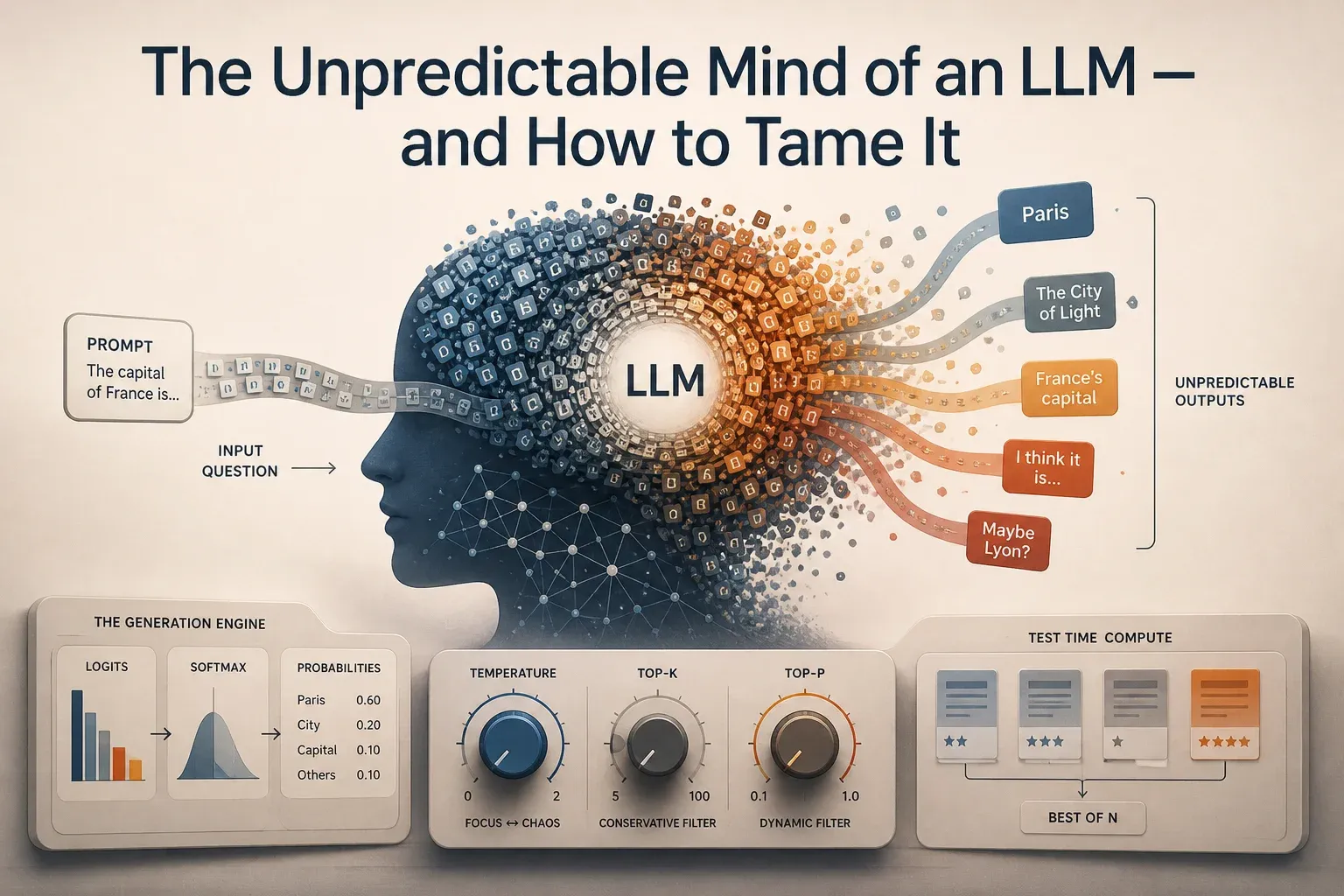
Imagine a colleague who gives a slightly different answer every time you ask the same question. Sometimes that’s a gift — fresh angles you hadn’t considered, a spark of creativity that solves a stale problem. Other times, it’s maddening. You needed a JSON object or a straight “Yes/No,” and you got a philosophical detour or a malformed string of text.

That’s the everyday reality of working with a Large Language Model (LLM). For many, the first instinct is to treat an LLM like a database: a place where facts are stored and retrieved. But LLMs don’t “know” answers in the way a relational database does. They don’t look up records; they hallucinate possibilities based on a probabilistic motor. This motor is the root of both their creative brilliance and their occasional, maddening inconsistency.

The Engine Room: From Logits to Tokens

To control the beast, you first have to understand how it thinks. When you give a prompt to an LLM, it doesn’t immediately spit out a word. It goes through a heavy mathematical computation to predict the very next piece of text, called a “token.”

Logits: The Raw Scores

At the final layer of the neural network, the model produces a long vector of numbers called logits. Each number corresponds to a token in the model’s vocabulary (which can be 100,000+ words, sub-words, or characters).

Logits are raw scores. A higher logit means the model “thinks” that token is more likely to come next. However, these numbers aren’t probabilities yet — they can be negative, and they don’t sum up to 100%. If “Apple” has a logit of 12.5 and “Banana” has a logit of 10.2, we know Apple is more likely, but we don’t know by how much.

The Softmax Transformation

To turn these raw scores into something usable, the model applies a mathematical function called Softmax. This function scales the logits into a probability distribution where every value is between 0 and 1, and the total sum is exactly 1 (or 100%).

$p*i = \frac{e^{x_i}}{\sum*{j} e^{x_j}}$

Once we have this distribution, we can see that “Apple” might have a 75% probability, while “Banana” has 20%, and “Car” has 5%.

Logprobs: The Scale of Precision

In AI engineering, you’ll often hear about logprobs (logarithms of probabilities). Why not just use the 0-100% scale?

The reason is a computer science problem called underflow. With a vocabulary of 100,000 tokens, many words have a probability so tiny (like 0.0000000001%) that a computer might round them down to zero, losing critical information. By working on a log scale, we turn these tiny decimals into more manageable negative numbers. Adding logprobs is also mathematically equivalent to multiplying probabilities, which is much faster and more stable for calculating the likelihood of a long sentence.

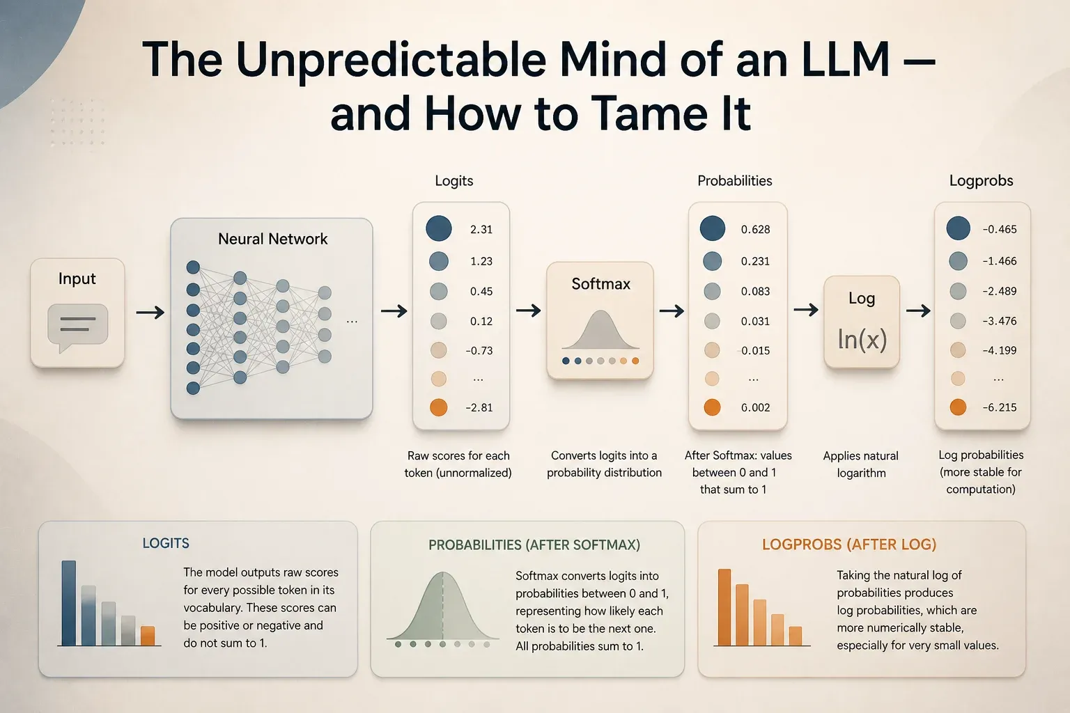Figure 1: From raw logits to normalized probabilities and finally stable logprobs - the hidden mathematical pipeline that shapes every token an LLM generates.

The Knobs of Control: Sampling Strategies

If we always picked the token with the absolute highest probability, the model would be “greedy.” While greedy sampling is predictable, it often lead to robotic, repetitive, and boring text. To make models feel “alive,” we introduce randomness. But how do we stop that randomness from turning into total chaos?

We use four primary knobs: Temperature, Top-K, Top-P, and the newer Min-P.

Temperature: The Focus vs. Chaos Knob

Temperature is a constant ($T$) that we divide the logits by before applying the Softmax.

• Low Temperature ($T < 1.0$): This “sharpens” the distribution. The most likely token gets even more probability, and the “long tail” of weird tokens gets squashed.
  • Use Case: Data extraction, code generation, or translation.
  • Example: If the model is 60% sure about the word “Paris,” at $T=0.1$, it might become 99% sure.
• High Temperature ($T > 1.0$): This “flattens” the distribution. It takes probability away from the leaders and gives it to the underdogs.
  • Use Case: Creative writing, brainstorming, or roleplaying.
  • Example: At $T=1.5$, “Paris” (60%) might drop to 40%, giving rare words like “The City of Light” a real shot at being picked.

[!TIP] Pro Engineering Tip: Setting Temperature to exactly 0 is a common convention for “greedy sampling.” Technically, you can’t divide by zero, so the hardware simply skips the math and picks the highest logit.

Top-K Sampling: The Conservative Filter

Top-K tells the model: “Only look at the top $K$ most likely words, and throw everything else away.”

If $K=50$, and the 51st word is “Elephant,” it doesn’t matter how high your Temperature is — “Elephant” will never be picked. This is a safety net that prevents the model from choosing complete gibberish (tokens with extremely low probability) just because the Temperature was high.

• Use Case: General chat where you want diversity but want to prevent the model from going “off the rails” into random character strings.

Top-P (Nucleus) Sampling: The Dynamic Filter

Unlike Top-K, which always looks at a fixed number of tokens, Top-P (or Nucleus sampling) looks at a dynamic number of tokens. It adds up the probabilities of the most likely words in descending order and stops as soon as the total hits $P$.

If $P=0.9$ (90%), and the top choice has a 95% probability, Top-P will only consider that one word. If the model is uncertain and the top choices are all around 5%, it might look at dozens of words to reach that 90% threshold.

• Use Case: Ideal for natural conversation. It allows the model to be creative when there are many valid ways to continue a sentence, but forces it to be precise when only one or two words make sense.
• Example Sentence: “The capital of France is…” -> Model is very certain, Top-P narrows to just “Paris.”
• Example Sentence: “Once upon a time, there was a…” -> Model is uncertain, Top-P expands the candidate pool to include “king,” “dragon,” “girl,” etc.

Min-P: The Noise Remover

A newer strategy gaining popularity is Min-P. Instead of a cumulative sum, Min-P sets a minimum threshold relative to the top token’s probability. If the top token has a 50% probability and Min-P is 0.1, only tokens with at least 5% (10% of 50%) probability are considered. This effectively filters out the “low-probability noise” that can sometimes cause models to trip over themselves.

See It In Action: Sampling Strategies Side-by-Side

Test Time Compute: “Thinking” Before Speaking

What if instead of tweaking how a single response is generated, you generated several and picked the best one? This is known as Test Time Compute. As the name suggests, you are spending more “compute” (processing power) at “test time” (inference) to get a better result.

Best-of-N (Rejection Sampling)

In this strategy, the model generates $N$ independent responses to the same prompt. Then, a second model (usually a Reward Model or a Verifier) scores each one. You only show the user the response with the highest score.

• Real World Success: Companies like Stitch Fix and Grab use reward models to pick the best output rather than relying on a single lucky roll of the dice.
• Performance Boost: OpenAI researchers found that using a verifier for math problems resulted in a performance boost equivalent to a 30x increase in model size. This means a small, fast model could potentially beat a massive, slow model just by generating multiple attempts and picking the best one.

Beam Search

While standard sampling picks one token at a time, beam search keeps track of the $B$ most promising sequences (the “beams”) simultaneously. At each step, it branches out from the current beams and keeps only the top $B$ paths that have the highest cumulative probability.

• Use Case: Highly structured tasks like Machine Translation. It’s less common in creative chat because it tends to lead to safe, generic-sounding results that lack “flavor.”

Self-Consistency

For math and logic, you can use Self-Consistency. You generate several responses (maybe 10) and then pick the answer that appears most frequently (majority voting).

• Example: If a model solves a math problem 10 times and gets “42” seven times and “41” three times, you pick “42.”

The Shadow Side: Hallucination and Inconsistency

If probabilistic outputs are a feature that allows for creativity, they are also a bug that causes hallucination and inconsistency. To build reliable AI, we must understand why the model “lies.”

The Self-Delusion Hypothesis (Snowballing)

Researchers at DeepMind and Stanford have explored a phenomenon called Snowballing Hallucination. Because LLMs generate text token-by-token, every word they say becomes part of their future “truth.”

Imagine you ask: “Is 9677 a prime number?” If the model gets a “lucky” roll and says “No,” but then follows up with “It’s divisible by 13,” it has committed to a lie. Even if the model “knows” 9677 isn’t divisible by 13, it will continue to output facts that support its initial wrong claim to maintain internal consistency. This is Self-Delusion: once a model makes a mistake, it often doubles down on it to justify the prefix.

The Training Gap (Mismatch in SFT)

Why does the model lie in the first place? One hypothesis is that we teach it to. During Supervised Fine-Tuning (SFT), models are trained on high-quality human responses. If a human labeler uses knowledge that the model doesn’t actually have in its weights, we are effectively teaching the model to “pretend” or “mimic” knowledge it doesn’t possess.

In production, when the model hits the edge of its knowledge, it does exactly what it was trained to do: it mimics the tone of a factual answer, even if the facts are missing.

Mitigation: Verifiers and Caching

How do we engineering around this?

• Fixing Sampling Variables: Locking the seed, temperature, and top-p values can help, but it’s not a silver bullet. Hardware differences (GPU types) can still cause tiny variations in floating-point math that lead to different outputs.
• Verification: As discussed in Test Time Compute, asking a second model to “check the work” of the first model is one of the most effective ways to kill hallucinations.
• Retrieval Augmented Generation (RAG): By providing the model with a “ground truth” document in its prompt, we narrow the probability distribution toward the facts in the text, leaving less room for the model to wander.

Conclusion: Engineering for Uncertainty

The dream of a perfectly predictable, deterministic LLM is a misunderstanding of how the technology works. If we wanted a deterministic machine, we’d use a calculator.

Probabilistic outputs aren’t a flaw — they are the mechanism behind every surprisingly good response, every clever piece of code, and every empathetic chat an LLM has ever given you.

As an AI engineer, your job isn’t to eliminate randomness, but to tame it.

• Dial down temperature when you need a surgeon’s precision.
• Turn to Top-P when you want a natural, human-like flow.
• Scale your Test Time Compute when the cost of being wrong is higher than the cost of a few extra tokens.

Control the randomness, and you control the future of your application.

References

1. Constrained Beam Search – Hugging Face Blog. A deep dive into forcing LLMs to follow specific grammars and constraints during sequence generation.
2. LLM Sampling Notes – Chip Huyen. A comprehensive guide to the probabilistic nature of modern language models and how to control them in production.