Machine Learning Engineer - 2

Thinking in Frequencies: Complex Numbers, Convolution, and Why Your Dense Matrix Was Never Really Dense

Aug 2, 2026

•

28 min read

AI-Generated Cover Image — Distributed Representations

🤖 Cover image generated by AI.

Part 3 of the series on Geometry, Topology, and the Future of Machine Learning Representation

There is a moment in most signal processing courses where the professor writes $e^{i\omega t}$ on the board and says something like “this is just a rotating vector in the complex plane” — and half the class nods while the other half writes it down and hopes to understand it later. If you were in the second half, this post is for you.

In the first blog, we argued that meaning in machine learning is stuck being represented as a static point — a vector with amplitude but no phase, a location with no dynamics. In the second, we saw how the brain sidesteps this by distributing representations across populations of neurons, using an algebra of binding and superposition rather than simple geometric proximity.

Now we go one level deeper. If signals are the right language for representation, and if that language involves complex exponentials — what does “frequency domain” actually mean, and why do complex numbers show up so naturally there? And once that foundation is in place, we’ll see how these ideas power some of the more interesting recent work in sequence modeling, specifically State Space Models like S4 and Mamba, where a single physical insight lets you flip between two completely different ways of computing depending on whether you’re training or running inference.

There’s also a beautiful algebraic puzzle sitting at the heart of all this: the statement that almost any dense real matrix is diagonalizable over the complex numbers. It sounds like dry linear algebra. It isn’t. It’s actually saying something deep about what “correlation” and “independence” even mean — and why complex numbers are the natural coordinate system for memory in a dynamical system.

Let’s get into it.

Part 1: Lets revisit, what is a Signal, Really?

Before complex numbers or Laplace transforms, let’s think about what we’re actually working with.

A signal is just a function of time. Your audio file, your EEG recording, the sequence of tokens fed into a language model — they’re all mappings from time (or position) to some value. The “value” could be a single number (a microphone reading), a vector (the hidden state of a neural network), or something higher-dimensional.

The simplest interesting signal is a pure sine wave: $u(t) = A \sin(\omega t + \phi)$ . Three numbers completely describe it — amplitude $A$ , angular frequency $\omega$ , and phase $\phi$ . The remarkable fact, which Fourier worked out in the early 1800s, is that any signal you will ever encounter in practice can be written as a (possibly infinite) sum of these pure sine waves. Different sines at different frequencies, amplitudes, and phases, added together.

This is why frequencies matter. A signal’s “frequency content” is just the recipe: which sines you need, and how much of each.

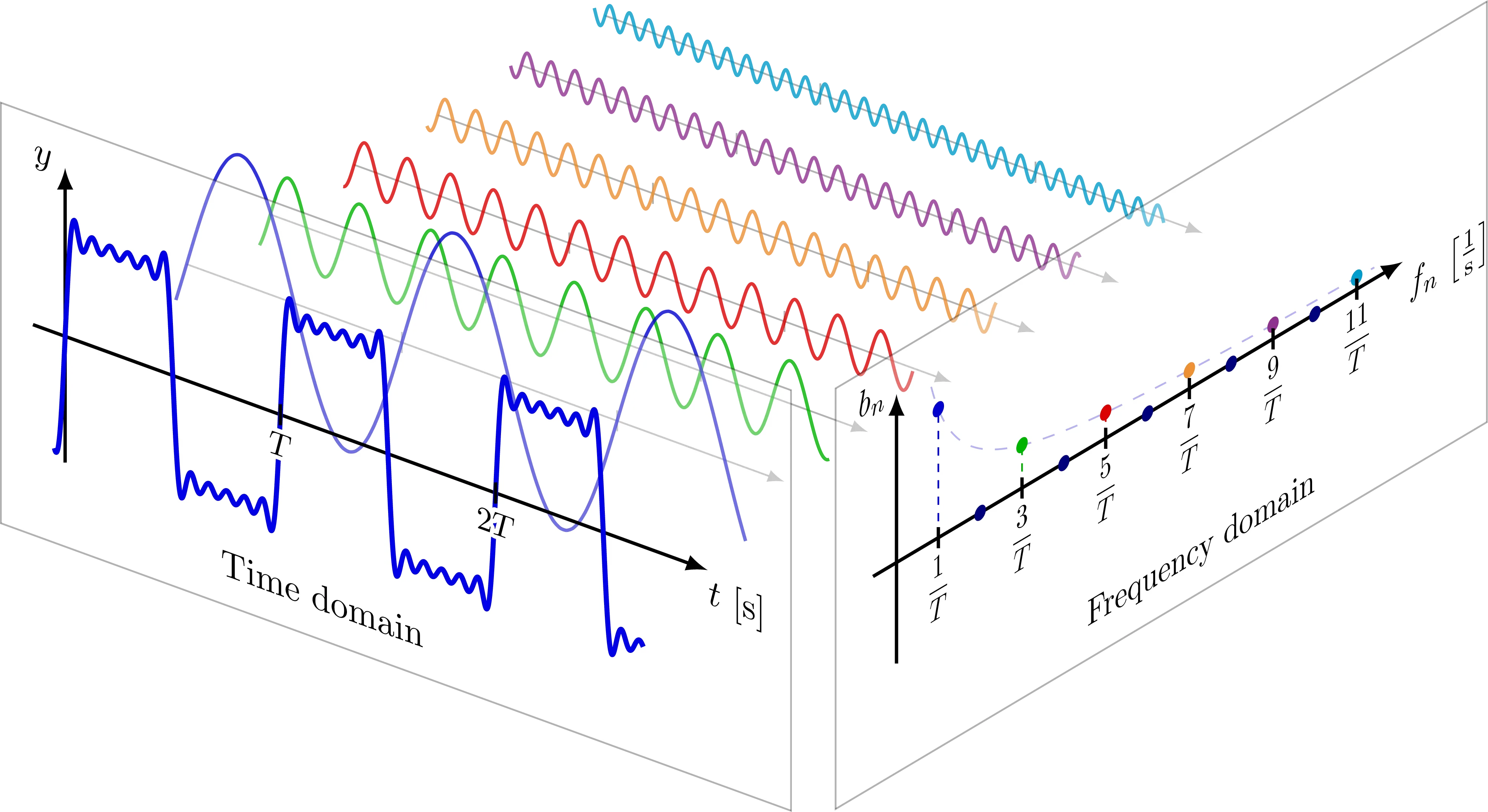Source: Duke Institute for Brain Sciences Methods Meetings Figure 1. Signal decomposition using the Fourier series.

But here is the awkward thing. Sines and cosines are clunky to work with algebraically. When you differentiate $\sin(\omega t)$ you get $\omega \cos(\omega t)$ , which is a different function. When you multiply two sines together you get a mess involving sum and difference frequencies. Every calculation turns into a trigonometric identity hunt.

Complex exponentials are the way out.

Part 2: $i$ is Not a Number — It’s a Rotation

Most of us first met $i = \sqrt{-1}$ as a bookkeeping trick for quadratic equations that had no real solutions. This framing, while historically accurate, is pedagogically unfortunate. It makes $i$ feel like a kludge.

Here is a better picture. Imagine you are standing at the point $(1, 0)$ on a 2D plane. Multiplying by $-1$ takes you to $(-1, 0)$ — you rotate $180°$ around the origin. Multiplying by $-1$ twice brings you back. So $-1$ is “rotate by $180°$ .”

Now ask: is there an operation that, applied twice, gives you “rotate by $180°$ ”? Yes — rotate by $90°$ . That operation is $i$ . Multiplying by $i$ is a quarter-turn counterclockwise.

$i \cdot (1, 0) = (0, 1)$ $i \cdot (0, 1) = (-1, 0)$

This is not a metaphor. It is literally what complex multiplication does geometrically. Any complex number $z = a + bi$ can be written in polar form as $z = r e^{i\theta}$ , where $r$ is its magnitude (distance from origin) and $\theta$ is its angle. Multiplying two complex numbers multiplies their magnitudes and adds their angles. Rotation composes by addition of angles.

Now go back to our sine wave. The signal $e^{i\omega t} = \cos(\omega t) + i \sin(\omega t)$ is a point spinning counterclockwise on the unit circle, completing one full revolution every $T = 2\pi/\omega$ seconds. The real part of that spinning point traces a cosine. The imaginary part traces a sine.

The beautiful thing: the derivative is trivial. $\frac{d}{dt} e^{i\omega t} = i\omega \cdot e^{i\omega t}$ . Differentiation is just multiplication by $i\omega$ . No change of function type, no trigonometric juggling. This is why physicists and engineers switched to complex exponentials the moment they learned them — every differential equation involving oscillations becomes dramatically simpler.

In signals, the imaginary component is not “fictitious.” It encodes the quadrature component — what a $90°$ -shifted copy of the signal looks like. If the real part tells you where the oscillator is (position), the imaginary part gives you the reference needed to reconstruct the instantaneous phase — and from that, which way the oscillation is heading. A purely real signal doesn’t let you distinguish a sine wave moving forward from one moving backward. The complex representation does.

Part 3: Can We Go Higher? The Question of a Third Representation

If complex numbers ( $\mathbb{C}$ ) extend the real line to 2D by adding one imaginary unit $i$ with $i^2 = -1$ , you might naturally ask: can we go further? Is there a “3D” version?

This is where things get genuinely surprising. Hamilton spent a decade trying to construct a 3D number system, assuming (reasonably) that the pattern would go $1 \to 2 \to 3$ dimensions. He failed. Eventually he realized the jump had to go to four dimensions — quaternions ( $\mathbb{H}$ ):

$q = a + bi + cj + dk$

where the three imaginary units satisfy $i^2 = j^2 = k^2 = ijk = -1$ , and the multiplication rules are:

$ij = k, \quad jk = i, \quad ki = j$ $ji = -k, \quad kj = -i, \quad ik = -j$

Crucially, quaternion multiplication is non-commutative: $ij \neq ji$ . This isn’t a flaw — it’s exactly what you need to represent 3D rotations, where “rotate around X then around Y” gives a different result than “rotate around Y then around X.” Quaternions are the native language of 3D rotation. Aerospace engineers, game developers, and roboticists use them constantly.

For signals, quaternionic representations appear in “vector sensor” processing — problems where your measurement has three spatial axes, like a 3D accelerometer, a magnetic field sensor, or polarized electromagnetic wave analysis. A quaternionic signal carries four coupled components that rotate together in 4D space.

The algebraic ladder doesn’t stop there. Octonions ( $\mathbb{O}$ ) give you eight dimensions, though they lose associativity and become harder to work with. Geometric Algebra (Clifford Algebra) is the systematic generalization: it lets you define “number systems” for $N$ -dimensional spaces where the algebra directly encodes geometric transformations — rotations, reflections, projections — as first-class algebraic operations.

Why Are These Representations Equivalent?

This question deserves a direct answer. When we say that a real signal can be represented as a complex exponential, or that a 3-axis measurement can be represented as a quaternion, we’re claiming the representations are equivalent. What does that mean?

The formal word is isomorphism. Two representations are isomorphic if there is a bijection between them that preserves the algebraic structure — you can convert back and forth, and all the relationships between elements are preserved.

A 2D real vector $(a, b)$ and a complex number $a + bi$ are isomorphic as vector spaces. The information content is identical. What changes is the algebraic structure you get for free: complex numbers come equipped with a multiplication rule that encodes rotation. When you multiply two complex numbers, you are automatically rotating and scaling — an operation that would require a matrix multiplication in the real vector space.

Rotation is the invariant. Whether you describe a circular orbit as “the point $(\cos\theta, \sin\theta)$ moving on the unit circle” (real 2D), or as ” $e^{i\theta}$ spinning on the unit complex circle” (complex 1D), the underlying physical motion is identical. The complex representation just makes the calculus simpler.

The same logic extends upward. The information in a unit quaternion encoding a 3D rotation is equivalent to a $3 \times 3$ rotation matrix or a pair of angles in Euler form. The representations are different languages for the same geometric object. You choose based on what computations you need to do efficiently.

In machine learning, this matters because choosing the right representational basis can turn an $O(N^2)$ computation into $O(N)$ — not by approximating, but by finding the natural coordinate system.

Part 4: System Dynamics and the Laplace Transform

Now let’s bring this into the territory of sequence models. The question is: if we want to model a system that has memory — that is, its current output depends not just on the current input but on everything that came before — what is the right mathematical language?

The answer from physics and control theory is differential equations.

Consider a simple model: the state of a system $x(t)$ evolves according to

$\dot{x}(t) = Ax(t) + Bu(t)$ $y(t) = Cx(t)$

where $u(t)$ is your input (say, a sequence of tokens) and $y(t)$ is your output. The matrix $A$ describes how the system’s internal state decays, grows, or oscillates on its own. $B$ projects the input into the state space. $C$ projects the state back to the output.

This is the continuous-time State Space Model. If $A$ were a scalar (say, $A = -\lambda$ ), the solution would be $x(t) = e^{-\lambda t} x(0) + \ldots$ — a decaying exponential. For matrix $A$ , the solution involves $e^{At}$ , the matrix exponential. The system’s behavior over time is entirely determined by the eigenvalues of $A$ .

This ODE setup is elegant but it’s hard to see what frequency components the system responds to. To understand that, we need to change domains.

The Laplace Transform: Moving to Frequency Space

The Laplace Transform takes a function of time and returns a function of a complex frequency variable $s$ :

$\mathcal{L}\{f(t)\} = F(s) = \int_{0}^{\infty} f(t)\, e^{-st}\, dt$

Why does this help? Because derivatives become multiplications. Specifically, $\mathcal{L}\{\dot{f}(t)\} = sF(s) - f(0)$ . If we assume the system starts at rest ( $x(0) = 0$ ), then differentiating in time is the same as multiplying by $s$ in the Laplace domain.

Applying this to our state equation:

$s X(s) = A X(s) + B U(s)$ $(sI - A) X(s) = B U(s)$ $X(s) = (sI - A)^{-1} B U(s)$

Substitute into the output equation:

$Y(s) = C(sI - A)^{-1} B \cdot U(s) = H(s) \cdot U(s)$

The term $H(s) = C(sI - A)^{-1}B$ is the Transfer Function. It is the system’s complete fingerprint in the frequency domain — it tells you, for every complex frequency $s$ , how much the system amplifies or attenuates that frequency. The poles of $H(s)$ (values of $s$ where the denominator blows up) correspond to the eigenvalues of $A$ , which are the system’s natural “resonant frequencies.”

Notice what happened: the complicated ODE, which couples the state’s past to its future through a differential relationship, becomes a simple algebraic equation $Y(s) = H(s) \cdot U(s)$ in the Laplace domain. The dynamics are “frozen” into the transfer function.

The Convolution Theorem: The Bridge Back

Here is the key theorem connecting frequency domain to time domain:

Convolution Theorem: Multiplication in the frequency domain corresponds to convolution in the time domain.

If $Y(s) = H(s) \cdot U(s)$ , then $y(t) = (h * u)(t)$ , where $h(t) = Ce^{At}B$ is the impulse response — the system’s output when you poke it with a Dirac delta at $t = 0$ .

In words: the system’s output is the input signal convolved with the impulse response. Convolution is just a weighted sum of shifted copies of the input, where the weights are given by $h$ .

$y(t) = \int_{0}^{t} Ce^{A(t - \tau)} B\, u(\tau)\, d\tau$

This integral looks expensive — for each output time $t$ , you are integrating over the entire past. But the Convolution Theorem gives you a shortcut: compute $H(s)$ , compute $U(s)$ (the Laplace transform of the input), multiply them, and invert. Once you discretize the system, this same idea carries over to the discrete Fourier domain: multiplication in frequency space becomes an FFT-based convolution — parallelizable over the entire sequence.

Part 5: SSMs — The System That Speaks Two Languages

This is where the physics meets modern deep learning in a genuinely elegant way.

The ODE above needs to be discretized before you can run it on a computer. Using the bilinear (Tustin) method, which is a numerically stable way of approximating the continuous dynamics:

$x_k = \bar{A} x_{k-1} + \bar{B} u_k$ $y_k = \bar{C} x_k$

where $\bar{A}, \bar{B}, \bar{C}$ are discretized versions of the continuous matrices. This is a linear recurrence — an RNN with a very specific weight-tying structure derived from the underlying ODE.

Now you have the same system expressed two ways:

Recurrent form: $x_k = \bar{A} x_{k-1} + \bar{B} u_k, \quad y_k = \bar{C} x_k$

Convolutional form: $\bar{K} = (\bar{C}\bar{B},\ \bar{C}\bar{A}\bar{B},\ \bar{C}\bar{A}^2\bar{B},\ \ldots), \quad y = \bar{K} * u$

These are not approximations of each other. They are mathematically identical — two descriptions of the same computation.

	Recurrent View	Convolutional View
Form	$x_k = \bar{A}x_{k-1} + \bar{B}u_k$	$y = \bar{K} * u$
Useful for	Inference / generation	Training
Parallelism	Sequential (must wait for $x_{k-1}$ )	Fully parallel (FFT)
Memory	$O(N)$ — just the current state	$O(L)$ — stores the kernel
Token cost	$O(1)$ per token	Precomputed

During training, you know the entire sequence upfront. You precompute the SSM kernel $\bar{K}$ and run the convolution in parallel using FFTs — this is $O(L \log L)$ for a sequence of length $L$ , far better than the $O(L^2)$ of attention. During inference, you discard the kernel and run the recurrence step by step, maintaining only the current state — $O(1)$ memory, regardless of sequence length.

The transfer function $H(s)$ is the conceptual bridge between these two modes. The poles of $H(s)$ are the eigenvalues of $A$ . The shape of $H(s)$ across the imaginary axis (at $s = i\omega$ ) is the frequency response — exactly which frequencies the model is sensitive to.

This is not a trick. It’s a consequence of the mathematical structure of linear time-invariant systems, developed over a century of control theory and signal processing. SSMs are importing that entire toolkit into sequence modeling.

Part 6: Rethinking Matrix Multiplication Itself

Let’s take a step back. The SSM story showed us that a specific computation — applying a linear system to a sequence — can be reframed in the frequency domain to go from $O(L^2)$ to $O(L \log L)$ . But this principle is more general than SSMs. It applies to the most fundamental operation in all of deep learning: matrix multiplication.

A standard linear layer computes $y = Wx$ where $W \in \mathbb{R}^{D \times D}$ and $x \in \mathbb{R}^D$ . That’s $O(D^2)$ operations. If $D = 4096$ (a typical hidden dimension in a modern LLM — not to be confused with the small state dimension $N$ from the SSM discussion above, which is usually 16–64), that’s sixteen million multiply-adds per layer per token. This is the computational bottleneck of deep learning.

The frequency domain suggests a different path.

The Circulant Special Case

Consider a matrix where each row is just a cyclic shift of the row above it:

$W = \begin{pmatrix} w_0 & w_1 & w_2 & w_3 \\ w_3 & w_0 & w_1 & w_2 \\ w_2 & w_3 & w_0 & w_1 \\ w_1 & w_2 & w_3 & w_0 \end{pmatrix}$

This is called a circulant matrix. It is dense — in general, every element is nonzero. But it has a hidden structure: every row contains the same information, just rotated.

Now apply the Convolution Theorem. Multiplying by a circulant matrix is equivalent to circular convolution with its first row. And circular convolution in the time domain is element-wise multiplication in the frequency domain. So:

$Wx = \mathcal{F}^{-1}\left(\mathcal{F}(w) \odot \mathcal{F}(x)\right)$

where $w$ is the first row of $W$ and $\odot$ is element-wise multiplication. The $O(D^2)$ matrix multiplication collapses to $O(D \log D)$ — one FFT, one element-wise multiply, one inverse FFT.

Three steps replace $D^2$ operations:

Project $x$ into the frequency domain (FFT): expose its spectral components.
Scale each component independently (element-wise multiply by $\hat{w}$ ): apply the transformation.
Mix back into the original domain (IFFT): reassemble the result.

This is the core pattern. The “mixing” step (the FFT/IFFT) is what makes a diagonal operation in frequency space correspond to a rich, non-trivial operation in the original space.

Generalizing: Any Orthogonal Basis Will Do

There is nothing sacred about the Fourier basis here. Any orthogonal transformation $\Phi$ defines the same pattern:

$y = \Phi^{-1}\left(\Lambda \odot\ \Phi x\right)$

where $\Lambda$ is a learned diagonal (element-wise scaling in the $\Phi$ -basis). This computes a specific class of linear transformations — exactly the matrices that are diagonalized by $\Phi$ . For the Fourier basis, that’s the circulant matrices. For the Laplace eigenbasis, that’s the matrices whose action is convolution with an exponential kernel — exactly what SSMs compute.

Other choices of $\Phi$ give you other transformation classes:

Hadamard / Walsh-Hadamard basis: Real-valued, computationally cheap (no multiplications needed, just additions/subtractions), captures certain kinds of local correlations.
Wavelet basis: Localized in both time and frequency — useful when signals have structure at multiple scales.
Legendre polynomial basis: The HiPPO framework uses this. The projection of a function onto Legendre polynomials is the optimal way to compress its history while preserving the ability to reconstruct it — which is why this specific basis shows up in SSMs designed for long-range memory.
Learned $\Phi$ : If you let $\Phi$ itself be a learnable unitary matrix, you recover the full expressivity of an arbitrary linear transformation, but you’ve constrained it to remain orthogonal during training — a useful inductive bias.

The general principle is this: a dense linear transformation can always be decomposed as “project into a basis, scale, mix back.” The basis chooses what structure is made explicit, and the element-wise scaling is where the learning happens.

FNet: Taking This Into Transformers

A 2021 paper called FNet made this concrete in a striking way. The authors replaced the entire self-attention sublayer in a BERT-style transformer with a fixed, unlearned 2D Fourier transform — applied once over the sequence dimension and once over the feature dimension.

No learned attention weights. No query-key dot products. No softmax. Just FFT.

The result: on standard NLP benchmarks, FNet reached 92% of BERT’s accuracy at 7× the speed on long sequences. The attention mechanism — the thing everyone thought was the secret sauce of transformers — turned out to be largely doing what a fixed Fourier mixing would do anyway. The frequency domain, applied across tokens, was already a decent approximation of “which parts of the sequence should talk to each other.”

This doesn’t mean attention is useless — the remaining 8% matters, and for tasks requiring precise token-to-token matching (like copying or lookup), learned attention is genuinely superior. But FNet reveals that a significant chunk of what attention does is just mixing — spreading information across positions — and you can get that for free with a fixed transform.

Why This Matters for VSAs — The Fixed Dimension Constraint

Here is where this connects to Vector Symbolic Architectures, and where the computational argument becomes a structural one rather than just an optimization.

In a standard neural network, linear layers are free to change dimension. An $N$ -dimensional input can be projected to an $M$ -dimensional output, where $M \neq N$ . The matrix $W \in \mathbb{R}^{M \times N}$ is the instrument of that change. The network learns to compress, expand, and reproject as needed.

VSAs don’t have this freedom. The entire point of a VSA is that the dimension $D$ is fixed across all operations. Binding, bundling, and unbinding all produce vectors of the same size. You superpose fifty concepts into the same $D$ -dimensional vector, and the superposition is interpretable precisely because the dimension didn’t grow. This is the property that makes VSAs holographic — each component participates in encoding everything.

But this creates a problem. If you can’t change dimension, you can’t use the standard toolbox of weight matrices. A weight matrix $W \in \mathbb{R}^{D \times D}$ does preserve dimension, but it costs $O(D^2)$ , and more importantly, applying an arbitrary $W$ to a VSA hypervector destroys the algebraic structure — after multiplication by $W$ , the result is no longer composable with other hypervectors via the binding operation in any meaningful way.

What you can do in a fixed-dimension, structure-preserving regime is exactly the spectral decomposition pattern:

$y = \Phi^{-1}\left(\Lambda \odot\ \Phi x\right)$

For FHRR and SVSA, the natural choice is the Fourier basis. Binding (element-wise complex multiplication in the spectral domain) is the dimension-preserving primitive. And Fourier mixing is how you “route” information between spectral components without leaving the hypervector algebra.

Concretely: if $x$ is a complex hypervector in the spectral domain (as in SVSA), then a “learned linear transformation” that respects the VSA structure looks like:

Element-wise multiply by a learned complex vector $\lambda$ (scale each frequency component). This is the binding-like operation — it shifts phases and modulates amplitudes per frequency.
Apply a fixed or learned orthogonal mixing (e.g., inverse FFT, then re-FFT in a rotated basis, or apply a Hadamard matrix). This lets different spectral components interact.

These two operations together span the same space as circulant matrix multiplication — a rich class of linear transformations, but constrained to preserve the VSA’s holographic structure.

This is not a limitation of VSAs. It is a feature. The constraint to dimension-preserving, structure-respecting transformations is what keeps the representations composable. You pay for expressivity in exchange for algebraic integrity. And the frequency domain is the natural arena for both the computation and the algebraic structure to coexist.

The punchline, put bluntly: in any regime where dimension is fixed and structure must be preserved — whether that’s an SSM’s hidden state, a VSA’s hypervector space, or a spectral sequence model — matrix multiplication is the wrong primitive. The right primitive is element-wise scaling in a frequency basis, followed by orthogonal mixing. They span the same class of computations (circulant / convolution operators), cost $O(D \log D)$ instead of $O(D^2)$ , and they respect the geometry of the space they’re operating in.

Part 7: The Dense Matrix That Was Never Really Dense

Here is the statement from the Mamba papers that deserves a proper unpacking:

“Almost all dense matrices over $\mathbb{R}^{N \times N}$ are diagonalizable over $\mathbb{C}$ , leading to the result that almost all dense real SSMs are equivalent to a diagonal complex SSM.”

Let’s build the intuition carefully.

What Does a Dense $A$ Matrix Actually Mean?

In an SSM, $A$ governs how the hidden state $x(t)$ evolves. If $A$ is dense — all entries potentially nonzero — that means every dimension of the state $x$ depends on every other dimension. When dimension 1 changes, it pulls on dimensions 2, 3, …, $N$ . It’s a fully coupled system.

Computationally, this is $O(N^2)$ per step. Conceptually, it means the “memory features” are all tangled up — you can’t say “feature 3 is tracking high-frequency components” independently of what feature 7 is doing.

The Eigenvalue Decomposition and Why Real Numbers Aren’t Enough

Any square matrix $A$ can potentially be written as $A = P \Lambda P^{-1}$ , where $\Lambda$ is diagonal and the columns of $P$ are the eigenvectors. In this eigenbasis, the dynamics decouple: each component evolves independently according to its own eigenvalue.

The catch: for a real matrix $A$ , the eigenvalues might be complex. Consider the simplest example, a $90°$ rotation matrix:

$R = \begin{pmatrix} 0 & -1 \\ 1 & 0 \end{pmatrix}$

This matrix is dense. The $x$ -coordinate depends on the $y$ -coordinate and vice versa — they’re coupled. Now try to find real eigenvectors. A real eigenvector $v$ would satisfy $Rv = \lambda v$ for some real $\lambda$ , meaning the matrix just scales $v$ without rotating it. But this matrix rotates everything. There is no real direction that stays put. So there are no real eigenvectors.

However, in the complex plane, there are. The eigenvectors are $(1, -i)$ and $(1, i)$ , with eigenvalues $i$ and $-i$ respectively. These are complex vectors pointing in “diagonal” directions in the 4-dimensional space of $(x_{\rm real}, x_{\rm imag}, y_{\rm real}, y_{\rm imag})$ . In this complex basis, the rotation matrix becomes:

$\Lambda = \begin{pmatrix} i & 0 \\ 0 & -i \end{pmatrix}$

Diagonal. The two complex components now evolve independently: one spins counterclockwise, one clockwise. The coupling is gone.

Why Complex Eigenvalues Always Come in Conjugate Pairs

For a real matrix $A$ , if $\lambda = a + bi$ is an eigenvalue with eigenvector $v$ , then $\bar{\lambda} = a - bi$ is also an eigenvalue with eigenvector $\bar{v}$ . Complex eigenvalues come in conjugate pairs, always.

This is not a coincidence. If $Av = \lambda v$ for a real matrix $A$ , taking the complex conjugate of both sides gives $A\bar{v} = \bar{\lambda}\bar{v}$ — since $A$ is real, $\bar{v}$ is automatically an eigenvector too, with eigenvalue $\bar{\lambda}$ . Complex eigenvalues of a real matrix are unavoidably paired. The conjugate pair together encode one real oscillation: the two complex exponentials $e^{(a+bi)t}$ and $e^{(a-bi)t}$ combine (via Euler’s formula) to give $e^{at}(C_1\cos bt + C_2\sin bt)$ — a real, damped oscillation.

The Normal Modes: Decoupling Without Losing Information

Think about a mechanical system: three masses connected by springs. If you poke one mass, all three wiggle in a complicated, coupled dance. The matrix describing their positions is dense.

But every such system has normal modes — specific collective motions where all masses move in a coordinated pattern. You might have one mode where all three masses move together left-right, another where the outer two move inward while the middle moves out, and so on. The remarkable property of these modes: if you excite one mode, the others don’t respond. They are independent.

The normal modes are the eigenvectors of the system matrix. In the normal mode basis, the dense matrix becomes diagonal. Each mode has its own eigenvalue — its natural frequency and decay rate.

In the real number world, the “rotational” modes (oscillations) are coupled into $2 \times 2$ blocks in the block-diagonal form. In the complex number world, each oscillation splits into two independent complex exponentials — one for each rotation direction. Everything becomes $1 \times 1$ blocks. Fully diagonal.

What Diagonalization Means for SSMs

In an SSM with a diagonal complex $A$ matrix, each element $x_i(t)$ of the state evolves according to its own scalar equation:

$\dot{x}_i = \lambda_i x_i + b_i u$

where $\lambda_i \in \mathbb{C}$ is the $i$ -th eigenvalue. These are completely independent. $x_1$ doesn’t know $x_2$ exists.

This gives you:

$O(N)$ computation instead of $O(N^2)$ — element-wise multiplication instead of matrix-vector product.
Clean interpretability — each hidden unit is tracking one “mode” of the input, characterized by a frequency and a decay rate encoded in $\lambda_i$ .
Stable parameterization — it’s easier to constrain the eigenvalues directly (keep them on or inside the unit circle for stability) when they’re explicit parameters rather than emergent properties of a full matrix.

But here’s the question that should be nagging you: if the original dense real SSM had all these correlations between state dimensions, and the diagonal complex SSM has none — are they still the same computation?

Yes. The state dimensions themselves are different in the two representations. In the original system, each dimension of $x$ might correspond to something physically interpretable, and they talk to each other. In the diagonal complex system, each dimension corresponds to a normal mode — a particular oscillatory pattern that spans the original dimensions. The transformation $P$ (the matrix of eigenvectors) mixes the original state dimensions into these modes, and $P^{-1}$ mixes them back.

The input-output behavior — given the same $u(t)$ , both systems produce the same $y(t)$ — is identical. The transfer function $H(s) = C(sI - A)^{-1}B$ is invariant under this change of basis. The correlations weren’t eliminated; they were absorbed into the projection matrices $B$ and $C$ , which now handle the job of mixing and unmixing the modes.

This is the punchline. A dense matrix represents a system where the “memory features” are defined in an arbitrary, coupled coordinate system. The complex diagonalization finds the natural coordinate system — the eigenbasis — where each feature is an independent oscillatory mode. The apparent “independence” of the diagonal form isn’t the system forgetting about correlations; it’s the system finding the perspective from which those correlations look like separate, non-interacting frequencies.

Putting It Together

Let me close with a picture that tries to connect everything.

A signal is a function of time. You can describe it as a sequence of values (the obvious way), or as a sum of complex exponentials at different frequencies (the Fourier/Laplace way). These are isomorphic — same information, different language. The complex language is better for calculus because differentiation becomes multiplication.

A dynamical system with memory can be described as an ODE, which in the Laplace domain becomes an algebraic equation involving the transfer function $H(s)$ . The convolution theorem tells you that the system’s output is the input convolved with the impulse response — and this convolution can be computed either sequentially (recurrent) or in parallel (convolutional/FFT), depending on what’s computationally convenient.

State Space Models are the implementation of this idea in machine learning. During training, they wear the convolutional hat: precompute the SSM kernel, run FFT-based convolution over the whole sequence in parallel. During inference, they switch to the recurrent hat: maintain a fixed-size state and update it one token at a time. The theoretical guarantee that these two modes are equivalent comes directly from the Convolution Theorem.

And the diagonal complex $A$ matrix is not a special case or an approximation. It’s the natural coordinate system for the dynamics. Moving from a dense real $A$ to a diagonal complex $A$ is the same as moving from “arbitrary mass positions” to “normal mode amplitudes” — a change of basis that decouples the computation without changing the physics. The fact that this requires complex numbers is not incidental: complex numbers are the native language of rotation and oscillation, and oscillation is how you maintain stable long-term memory in a linear system.

The frequency domain isn’t just a mathematical tool. It’s the coordinate system where the problem has its simplest form.

Next in this series: we’ll go deeper into Vector Symbolic Architectures — specifically, how the element-wise complex multiplication + Fourier mixing pattern developed here becomes the foundation for binding, superposition, and algebraic inference in hypervector spaces, and why this structure has surprising resonances with the brain’s gamma-band synchronization and theta-gamma cross-frequency coupling.

Acknowledgments / Further Reading:

Albert Gu’s S4 paper and thesis are the primary source for the SSM treatment here. The HiPPO paper is essential context for why the $A$ matrix takes the form it does.
Lee-Thorp et al., FNet: Mixing Tokens with Fourier Transforms (2021) — the paper that showed FFT can replace attention and still reach 92% of BERT performance.
For the general theory of structured matrices and fast transforms: Dao et al., Monarch: Expressive Structured Matrices for Efficient and Accurate Training (2022) is an excellent entry point.
For Laplace transforms and transfer functions from first principles: Oppenheim & Willsky, Signals and Systems.
For geometric algebra as a framework for higher-dimensional signal representations: Hestenes, New Foundations for Classical Mechanics.
For quaternionic signal processing: Bülow’s dissertation on hypercomplex signal representations.

Author note: I have also used LLMs for writing, but the core ideas, technical direction, and learning are my own. The mathematical equations explaining each of the matrix multiplications or the state equations are also generated using LLMs.