Contributors: Ashwini Rao

Understanding & Working with 3D Point Cloud Data

This notebook is geared toward learners and practitioners looking to understand and work with 3D point cloud data using Python.

KITTI Continuous Point Cloud Visualization

Introduction

What is a Point Cloud ?

A distinct collection of points in a 3D space is called a point cloud. A digital representation of an object or environment is created from these points, which are typically captured by means of technologies like LiDAR (Light Detection & Ranging), 3D scanners, or radar. Each point in the cloud has a cartesian coordinate (X, Y, Z) and may also have additional values like color or intensity etc.

Point clouds are a way to represent 3D shapes and structures, providing a digital representation of the real world. Software for photogrammetry can also make these.

Common Usecases

• 3D Modeling Softwares
• Digital Twin
• Geo Survey & Mapping
• Urban Planning
• Automotive Industry

Other 3D Representations

Source: adioshun.gitbooks.io

• 3D Mesh: A digital representation of a 3D object made up of polygons, mainly triangles and quadrilaterals. An object's shape in 3D is defined by its collection of vertices or lines that connect vertices and faces, or polygons.

• Voxels: The abbreviation "volume pixel" refers to a three-dimensional point in a 3D grid that represents a volume in three dimensions. For 3D data, it is comparable to a pixel in a 2D image. Numerous domains, including 3D modeling, medical imaging, and scientific visualization, frequently use voxels.

• Depth Maps: An image or image channel that gives information about the distance of objects in a scene from a viewpoint is known as a "depth map" in computer graphics and computer vision. In essence, it allows the display of 3D objects or the fabrication of 3D illusions by encoding 3D depth information into a 2D image.

LiDAR Sensors

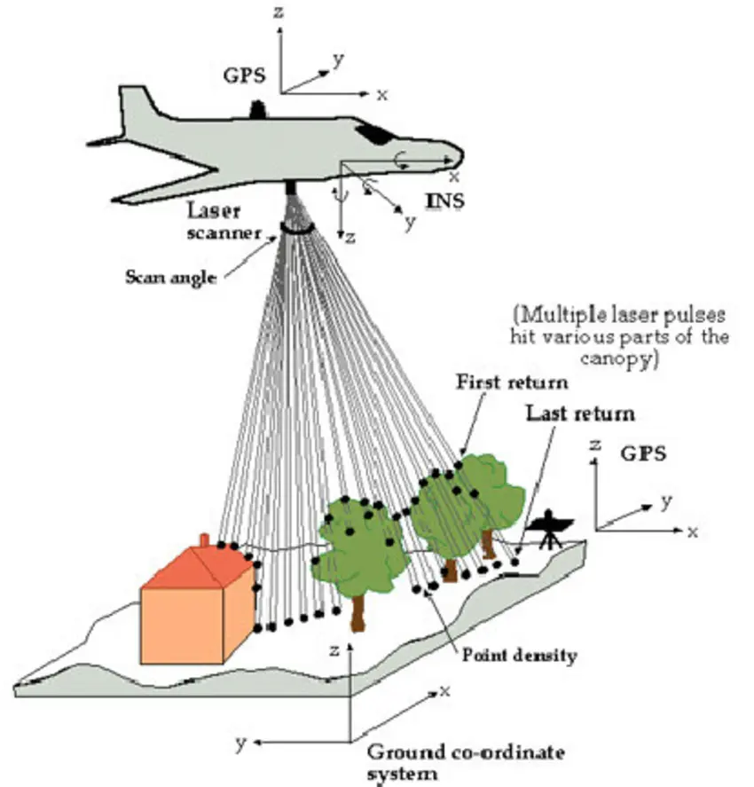
Aerial LiDAR

Airborne lidar, also known as airborne laser scanning, is the process of creating a 3-D point cloud model of the landscape using a laser scanner mounted on an aircraft while it is in flight. This technique has supplanted photogrammetry as the most precise and thorough way to create digital elevation models at the moment.

Below we can see the Aerial LiDAR setup & sample data collected from it:

It has applications in:

• Mapping and Surveying
• Urban Planning
• Transportation Management
• Disaster Management
• Environmental Monitoring
• Agriculture
• Mining & Construction

Rotating LiDAR

Rotating LiDAR (Light Detection and Ranging) is a type of 3D sensor that uses spinning laser beams to scan the surrounding environment. It uses a mechanical spinning mechanism to rotate its laser(s), typically on a horizontal axis (e.g., 360°).

Below we can see the Rotating LiDAR:

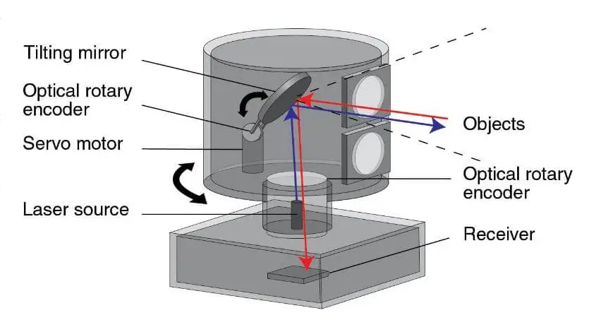
Sample data collected from it:

Rotating Lidar Sample Data from KITTI

It has applications in:

• Autonomous Driving
• Robotics

Data Formats

A data format defines how data is structured, stored, and interpreted by computers or software applications. Data formats vary widely depending on their use cases, such as text, images, audio, video, or geospatial information. Each format typically includes a set of rules for encoding the data and may also contain metadata to describe the content. There are several data formats to store 3d data which we will be looking into.

PCAP

Packet Capture files are commonly used to capture network traffic but they are also used in some LiDAR sensors to store their data. A PCAP file typically contains individual frames of point cloud data, each representing a scan from sensor. It stores raw point cloud data. The exact data format can vary from sensor to sensor. Using sensor specific or general tools we can convert these PCAP files to other formats like .las.

LAS / LAZ

Lidar point cloud data can be interchanged and archived using the LAS (LASer) file format. The American Society for Photogrammetry and Remote Sensing (ASPRS) established this open, binary format. The format is widely used and regarded as an industry standard for lidar data. Used across different softwares, geographic information systems (GIS), remote sensing & 3D modeling.

LAZ is a lossless compression of the LAS format. Used for efficient storage of the data.

Point Records Format:

Points are stored sequentially. A point format describes the dimensions stored for each point in the record.

Name	Description
X, Y, Z	Raw values are scaled and offsetted to get the X, Y, Z coordinates.
Intensity	The intensity value is the pulse return magnitude.
Return Number	Numerous returns may occur from a particular output laser pulse, and each one needs to be identified in order of return. It will start from one & can go upto five.
Number of Returns	Total number of returns for a given pulse. It can go upto five for a pulse.
Scan Direction Flag	The direction that the scanner mirror was moving at the moment of the output pulse.
Edge of Flight Line	It has a value of 1 only when the point is at the end of a scan. Last point before a scan line switches course.

Let's use laspy package to load a .las file & visualize the point cloud data.

Tool: laspy

import laspy
import numpy as np

# file path
FILE_PATH = "./images/sample_data/sample_0.las"

# read data
las = laspy.read(FILE_PATH)
print(las)

<LasData(1.2, point fmt: <PointFormat(1, 0 bytes of extra dims)>, 6826152 points, 0 vlrs)>

# Access file header
print(f"File Header: {las.header}")

# Point Records
print(f"# Points: {las.header.point_count}")

# Point Format & Dimensions
print(f"Point Format: {las.point_format.id}")
print(f"Point Dimensions: {list(las.point_format.dimension_names)}")

File Header: <LasHeader(1.2, <PointFormat(1, 0 bytes of extra dims)>)>
# Points: 6826152
Point Format: 1
Point Dimensions: ['X', 'Y', 'Z', 'intensity', 'return_number', 'number_of_returns', 'scan_direction_flag', 'edge_of_flight_line', 'classification', 'synthetic', 'key_point', 'withheld', 'scan_angle_rank', 'user_data', 'point_source_id', 'gps_time']

# Sample Point
print(f"Sample Point: {las.points[0].__dict__}")

Sample Point: {'array': np.void((36064535, 591139394, 76446, 136, 9, 2, 24, 3, 23207, 364254.77380318934), dtype=[('X', '<i4'), ('Y', '<i4'), ('Z', '<i4'), ('intensity', '<u2'), ('bit_fields', 'u1'), ('raw_classification', 'u1'), ('scan_angle_rank', 'i1'), ('user_data', 'u1'), ('point_source_id', '<u2'), ('gps_time', '<f8')]), 'point_format': <PointFormat(1, 0 bytes of extra dims)>, 'sub_fields_dict': {'return_number': ('bit_fields', SubField(name='return_number', mask=7)), 'number_of_returns': ('bit_fields', SubField(name='number_of_returns', mask=56)), 'scan_direction_flag': ('bit_fields', SubField(name='scan_direction_flag', mask=64)), 'edge_of_flight_line': ('bit_fields', SubField(name='edge_of_flight_line', mask=128)), 'classification': ('raw_classification', SubField(name='classification', mask=31)), 'synthetic': ('raw_classification', SubField(name='synthetic', mask=32)), 'key_point': ('raw_classification', SubField(name='key_point', mask=64)), 'withheld': ('raw_classification', SubField(name='withheld', mask=128))}, 'scales': array([0.01, 0.01, 0.01]), 'offsets': array([-0., -0., -0.])}

Scaling of the Points:

X, Y, and Z scale factors: The double floating point value in the scale factor fields is used to scale the associated X, Y, and Z long values in the point records. To obtain the real X, Y, or Z coordinate, multiply the X, Y, Z coordinates with the associated scale factors. If, for instance, the X, Y, and Z coordinates are intended to have two decimal points, then each scale factor will have the value 0.01.

X, Y, and Z offset: The overall offset for the point records should be set using the offset fields. These figures will typically be zero, however in some circumstances, the point data's resolution might not be sufficient for a particular projection method. It should always be assumed, nevertheless, that these figures are in use. Therefore, multiply the point record X by the X scale factor, then add the X offset to scale a given X from the point record.

X coordinate = (Xrecord * Xscale ) + Xoffset
Ycoordinate = (Yrecord * Yscale ) + Yoffset
Zcoordinate = (Zrecord * Zscale ) + Zoffset

def get_scaled_points(las: laspy.LasData) -> tuple[np.ndarray, np.ndarray, np.ndarray]:
    return np.vstack((las.X, las.Y, las.Z)).transpose() * las.header.scales + las.header.offsets

# Scale the points
points = get_scaled_points(las)
print(f"Shape: {points.shape}")
print(f"Points Range: {np.min(points, axis=0)} - {np.max(points, axis=0)}")
print(f"Range in header: {las.header.mins} - {las.header.maxs}")

Shape: (6826152, 3)
Points Range: [3.60513270e+05 5.90901878e+06 7.55820000e+02] - [3.6266162e+05 5.9113955e+06 8.0217000e+02]
Range in header: [3.60513270e+05 5.90901878e+06 7.55820000e+02] - [3.6266162e+05 5.9113955e+06 8.0217000e+02]

Farthest Point Sampling VS Random Sampling

# Plot the data
from lexper.utils.plotting import get_figure, plot_point_cloud

# There are a lot of points, we will sample a fixed set of points and plot the data
# For this we will use Farthest Point Sampling
def farthest_point_sampling(points: np.ndarray, k: int) -> tuple[np.ndarray, np.ndarray]:
    """
    Perform Farthest Point Sampling (FPS) on a point cloud.

    Args:
        points (np.ndarray): Input point cloud of shape (N, 3).
        k (int): Number of points to sample.

    Returns:
        sampled_points (np.ndarray): Sampled point cloud of shape (k, 3).
        sampled_indices (np.ndarray): Indices of sampled points in the original array.
    """
    N = points.shape[0]
    sampled_indices = np.zeros(k, dtype=int)
    distances = np.ones(N) * 1e10

    # Start with a random point
    farthest = np.random.randint(0, N)
    for i in range(k):
        sampled_indices[i] = farthest
        centroid = points[farthest, :3]
        dist = np.sum((points - centroid) ** 2, axis=1)
        distances = np.minimum(distances, dist)
        farthest = np.argmax(distances)

    sampled_points = points[sampled_indices]
    return sampled_points, sampled_indices


def generate_circle_points(n=50):
    theta = np.linspace(0, 2 * np.pi, n)
    x = np.cos(theta)
    y = np.sin(theta)
    z = np.ones_like(x)
    return np.stack((x, y, z), axis=1)


# Generate Random Points
example_points = generate_circle_points()
# Visualize these points
fig = get_figure()
plot_point_cloud(data=example_points, name="Raw Points", fig=fig, point_size=5)
fig.show()

n_points = 6
# Random Point Sampling
choices = np.random.choice(example_points.shape[0], size=n_points, replace=False)
randomly_sampled = example_points[choices]
# Farthest Point Sampling
farthest_points, _ = farthest_point_sampling(example_points, n_points)
# Compare
fig = get_figure(rows=1, cols=2)
plot_point_cloud(data=randomly_sampled, name="Randomly Sampled", fig=fig, row=1, col=1, point_size=5)
plot_point_cloud(data=farthest_points, name="Farthest Sampled", fig=fig, row=1, col=2, point_size=5)
fig.show()

We can see above that the randomly sampled points are spreaded out but in case of farthest point sampling the points are spread out covering the circle region.

Visualization

# Shift & Scale the points
scaled_points = points - las.header.mins

# First randomly sample some points
choices = np.random.choice(scaled_points.shape[0], size=50000, replace=False)
sampled_points = scaled_points[choices]

# Sample points
sampled_points, sampled_indexes = farthest_point_sampling(sampled_points, 20000)

fig = get_figure()
plot_point_cloud(data=sampled_points, name="Sample 0", fig=fig)
fig.show()

PLY

The Stanford Triangle Format and the Polygon File Format are other names for the PLY computer file format. Storing three-dimensional data from 3D scanners was its primary function. Among the various properties that can be saved are color and transparency, texture coordinates, surface normals, and data confidence values.

A collection of vertices, faces, and other elements that can be assigned characteristics like color and normal direction is referred to as an object in the PLY format.

The format of a standard PLY file is as follows:

• Header
  • Each type of element is described along with its name (ex: "edge"), how many of these elements there are in the object, and a list of the various attributes associated with the element. It also specifies if the file is binary or ASCII.
• Vertex List
  • The vertex list contains the actual 3D points, one per line, along with any associated properties (like color etc.)
• Face List
  • The face list defines polygonal surfaces (typically triangles) by referencing the indices of vertices defined above.
• (lists of other elements)

Tool: Open3D

import numpy as np
import open3d as o3

# Read File
FILE_PATH = "./images/sample_data/sample_1.ply"

ply = o3.io.read_point_cloud(FILE_PATH)
ply

PointCloud with 134536 points.

# Sample Points
print(np.asarray(ply.points)[:5])

[[-15.61418152  39.51490784   2.21499991]
 [-15.64233303  39.52183533   2.19350004]
 [-15.60787392  39.50787354   2.19712496]
 [-15.66040039  39.52479935   2.21700001]
 [-15.54650211  39.48743439   2.20106244]]

Visualization

# Plot the data
from lexper.utils.plotting import get_figure, plot_point_cloud

points = np.asarray(ply.points)[:, :3]
points = points - np.min(points, axis=0)

# Sample points
sampled_points, sampled_indexes = farthest_point_sampling(points, 20000)

fig = get_figure()
plot_point_cloud(data=sampled_points, name="Sample 1", fig=fig)
fig.show()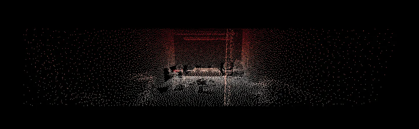

Voxelization

The voxel grid is another geometry type in 3D that is defined on a regular 3D grid, whereas a voxel can be thought of as the 3D counterpart to the pixel in 2D.

from open3d.web_visualizer import draw

voxel_size = 0.1  # Set voxel size (meters)
downsampled_ply = ply.voxel_down_sample(voxel_size=voxel_size)
voxel_grid = o3.geometry.VoxelGrid.create_from_point_cloud(downsampled_ply, voxel_size=voxel_size)
draw([voxel_grid])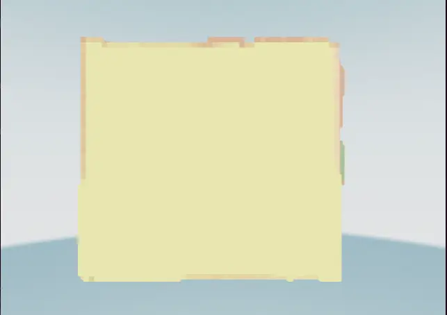

BIN

Most of the publicly available datasets are storing the point cloud data in .bin files -- typically as a sequence of floats or doubles representing point coordinates (x, y, z), intensity etc. It's easier to process while training ML models.

Tool: Numpy

import numpy as np

# KITTI Dataset File
FILE_PATH = "./images/sample_data/sample_2.bin"

# Read data - (X, Y, Z, Intensity)
bin  = np.fromfile(FILE_PATH, dtype=np.float32).reshape((-1, 4))
print(f"Points Shape: {bin.shape}")

Points Shape: (115384, 4)

# Sample points
print("Sample Points: ")
print(bin[:3])

Sample Points: 
[[1.8324e+01 4.9000e-02 8.2900e-01 0.0000e+00]
 [1.8344e+01 1.0600e-01 8.2900e-01 0.0000e+00]
 [5.1299e+01 5.0500e-01 1.9440e+00 0.0000e+00]]

Visualization

# Plot the data
from lexper.utils.plotting import get_figure, plot_point_cloud

fig = get_figure()
plot_point_cloud(data=bin[:, :3], name="Sample 2", fig=fig)
fig.show()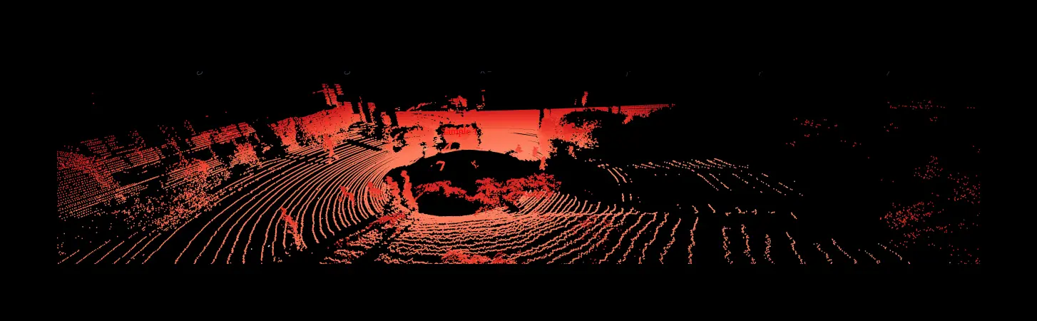

Famous Datasets

• Indoor RGB-D / 3D Scene Datasets

  • SUN RGBD
    • RGB-D images with 3D bounding box annotations
  • ScanNet
    • RGB-D scans, semantic & instance labels

• Autonomous Driving Datasets

  • KITTI
    • Benchmark classic, stereo, LiDAR, 3D bounding boxes
  • Waymo
    • High-quality LiDAR + multiple cameras, huge scale
  • NuScenes
    • 360° LiDAR + camera, radar, annotations, 10 classes

References

• What is point cloud data ?
• About LAS / LAZ Dataformat
• LAS Specification
• PLY Specifications